Hi everyone and happy Wednesday! Today we are going to look at how to solve inequalities with 2 variables. You may hear this in your class as “Simultaneous Inequalities” or “Systems of Inequalities,” all of these mean the same exact thing! The key to answering these types of questions, is to know how to graph inequalities and to know that the solution is always found where the two shaded regions overlap each other on the graph. We’re going to go over an example one step at time, then there will be practice questions at the end of this post that you can try on your own. Happy calculating! 🙂
How to Solve Inequalities with 2 Variables:
Just to review, when graphing linear inequalities, remember, we always want to treat the inequality as an equation of a line in form….with a few exceptions:
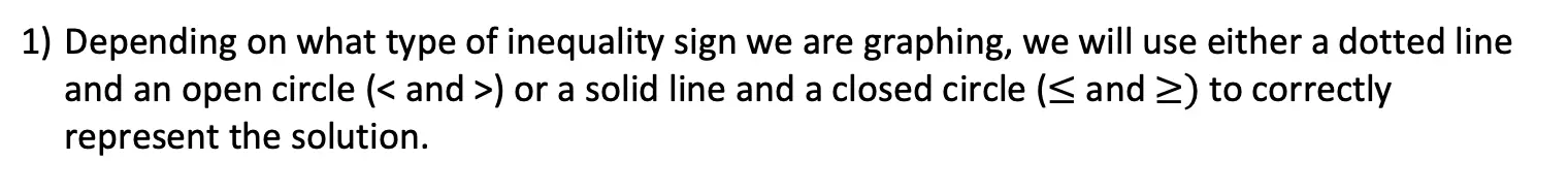
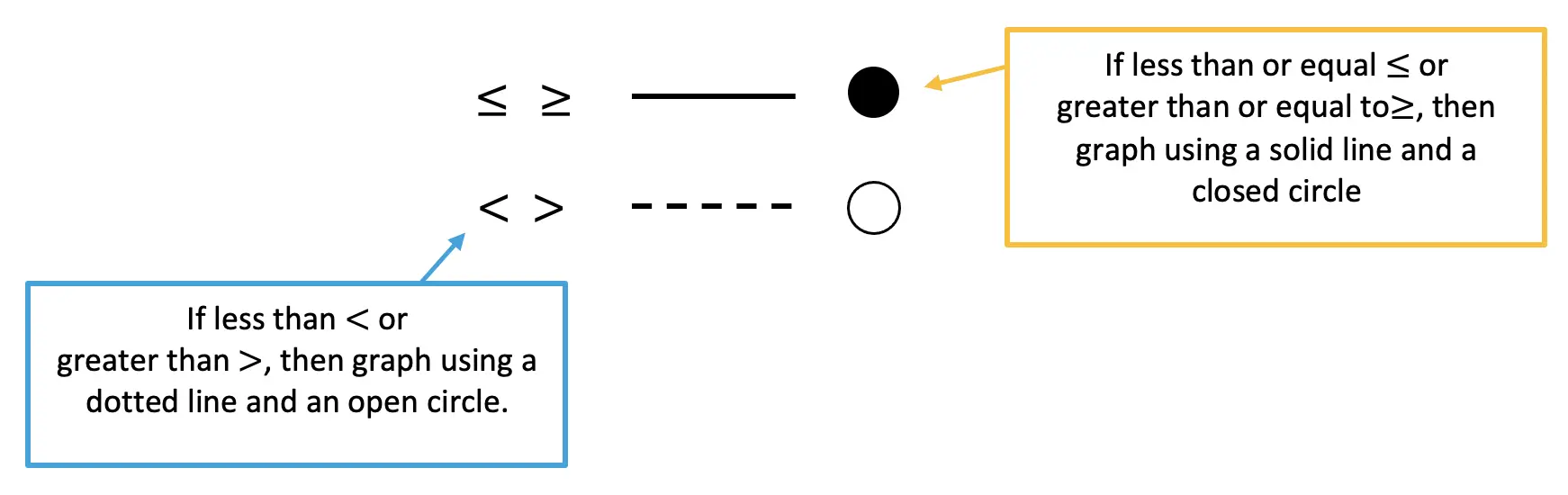
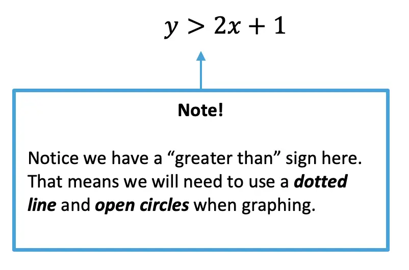
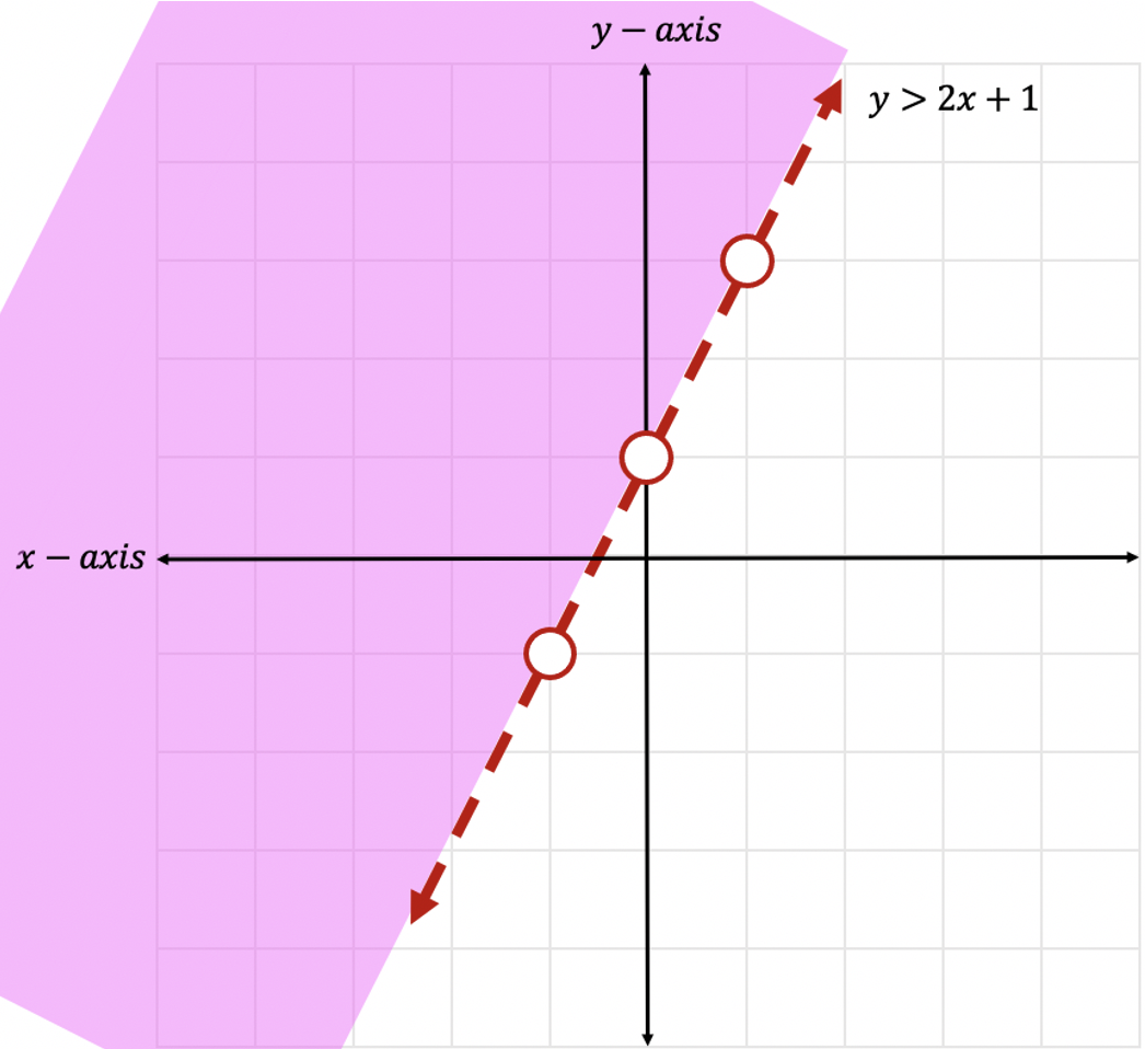
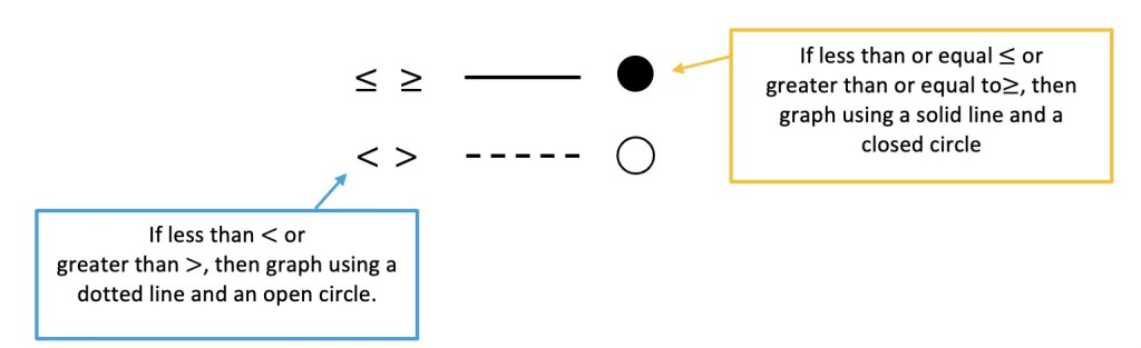
1)Depending on what type of inequality sign we are graphing, we will use either a dotted line and an open circle (< and >) or a solid line and a closed circle (> or <) and to correctly represent the solution.
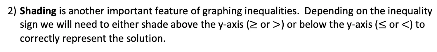
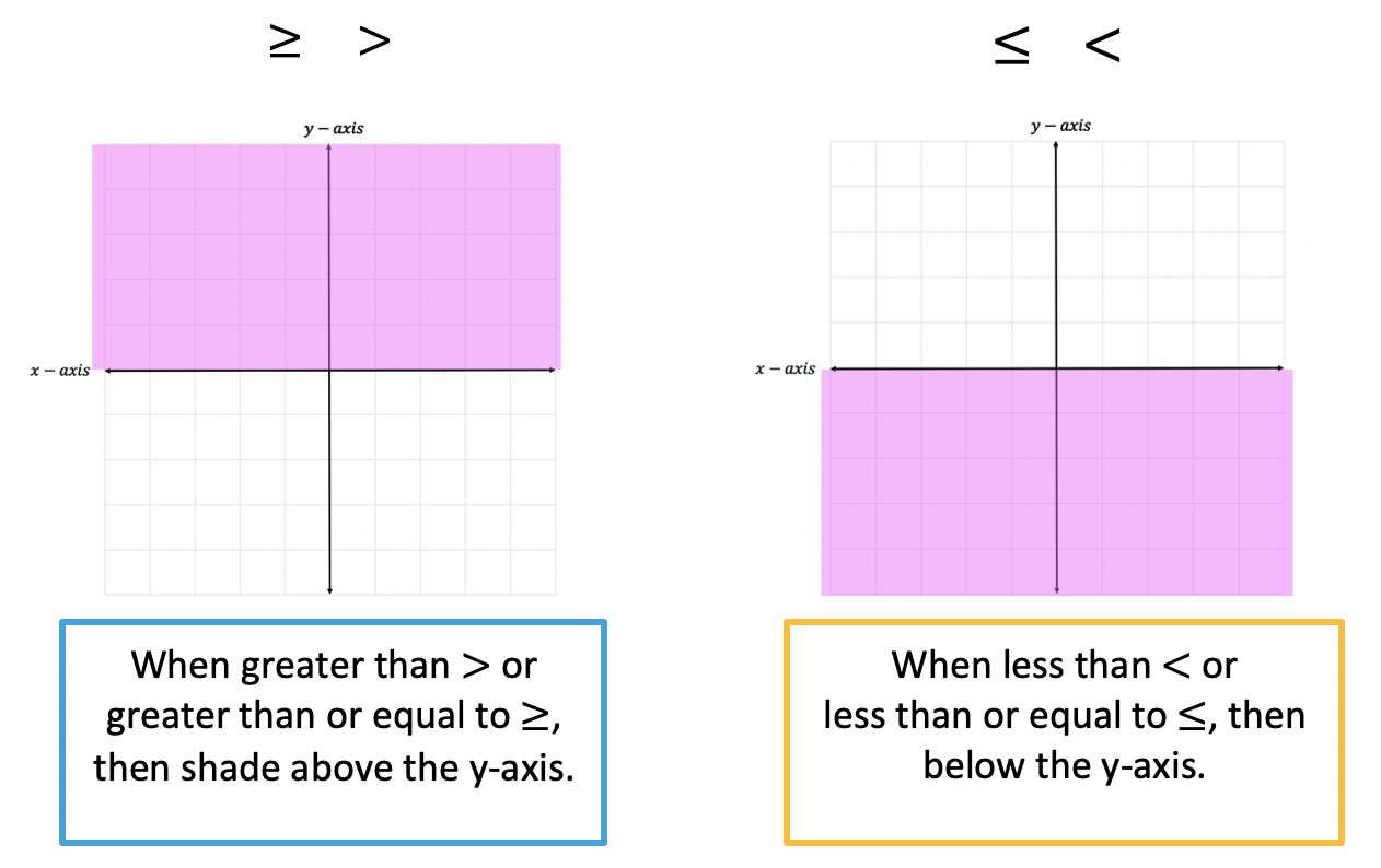
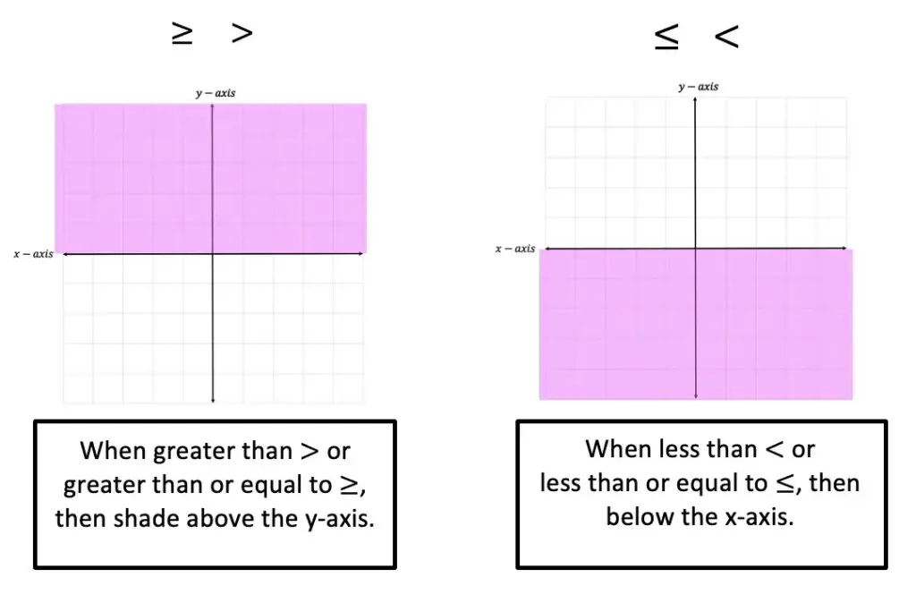
2) Shading is another important feature of graphing inequalities. Depending on the inequality sign we will need to either shade above the x-axis ( > or > ) or below the x-axis ( < or < ) to correctly represent the solution.
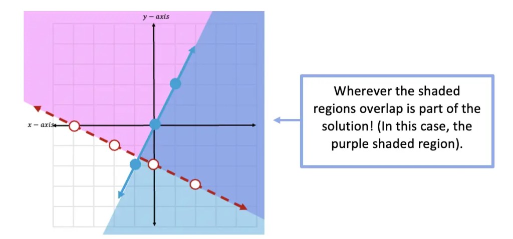
3) Solution: To find the solution of a system of inequalities, we are always going to look for where the shaded regions of both inequalities overlap.
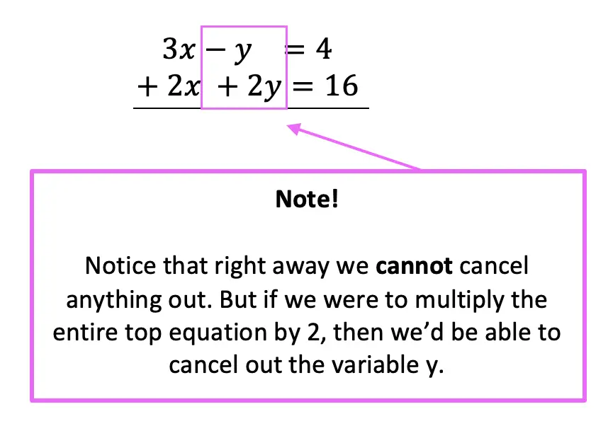
Now that we know the rules, of graphing simultaneous inequalities, let’s take a look at an Example!
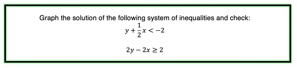
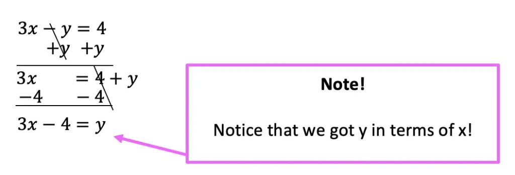
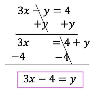
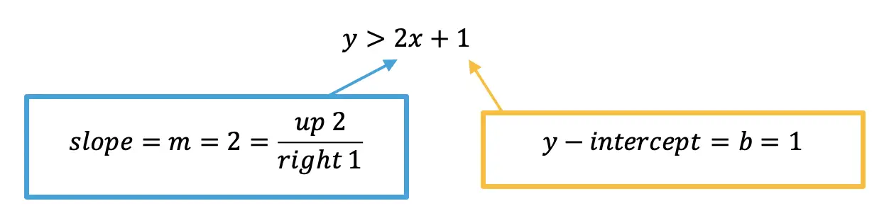
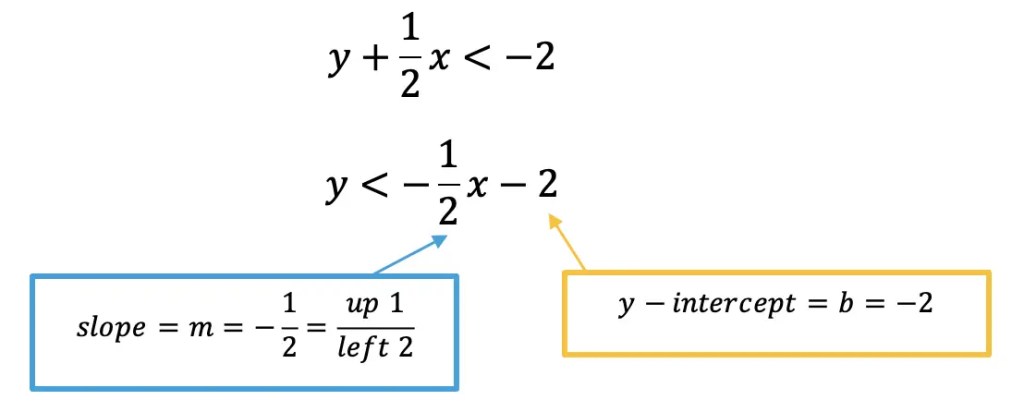
Step 1: First, let’s take our first inequality, and get it into y=mx+b form. To do this, we need to move .5x to the other side of the inequality by subtracting it from both sides. Once we do that, we can identify the slope and the y-intercept.
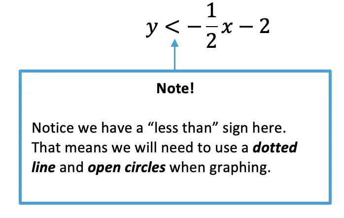
Step 2: Before graphing, let’s now identify what type of inequality we have here. Since we are working with a < sign, we will need to use a dotted line and open circles when graphing.
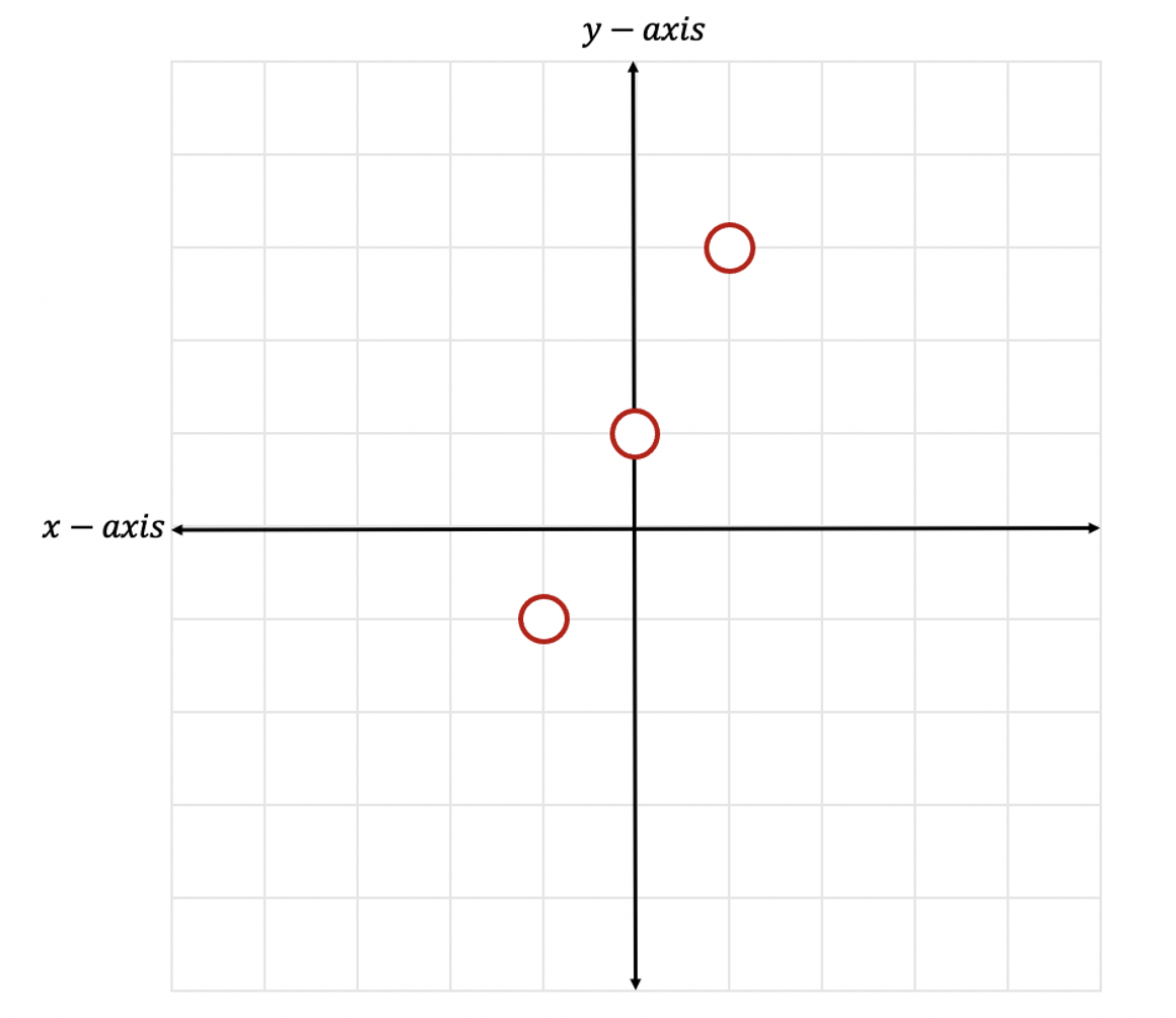
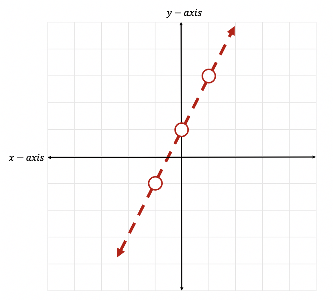
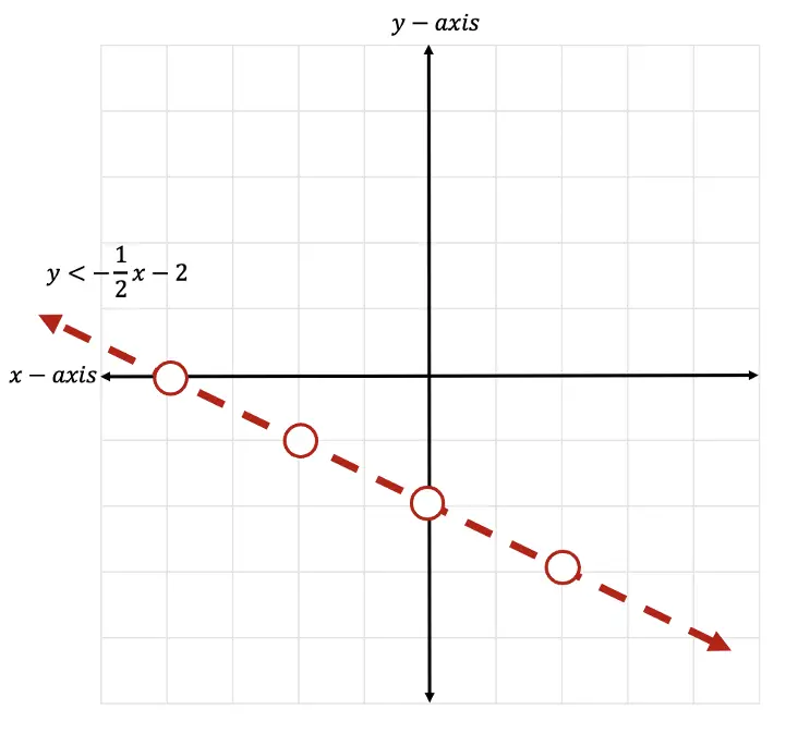
Step 3: Now that we have identified all the information we need to, let’s graph the first inequality below:
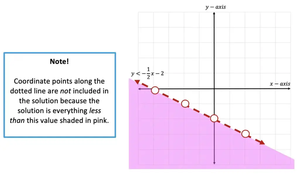
Step 4: Now it is time for us to shade our graph, since this is an inequality, we need to show all of our potential solutions with shading. Since we have a less than sign, <, we will be shading below the x-axis. Notice all the negative y-values below are included to the left of our line. This is where we will shade.
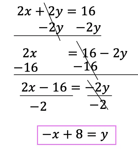
Step 5: Next, let’s start graphing our second inequality! We do this by taking the second equation, and getting it into y=mx+b form. To do this, we need to move 2x to the other side of the inequality by adding it to both sides. Then we can simplify the inequality even further by dividing out a 2.
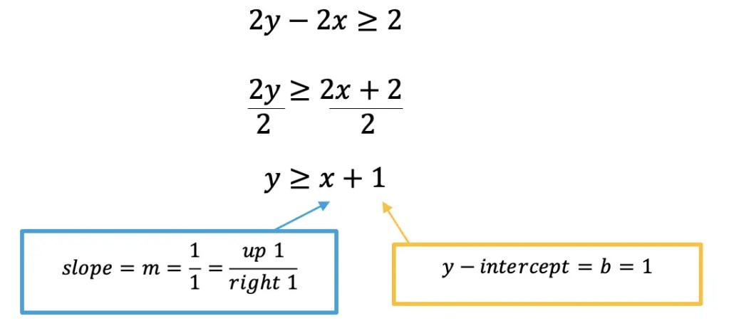
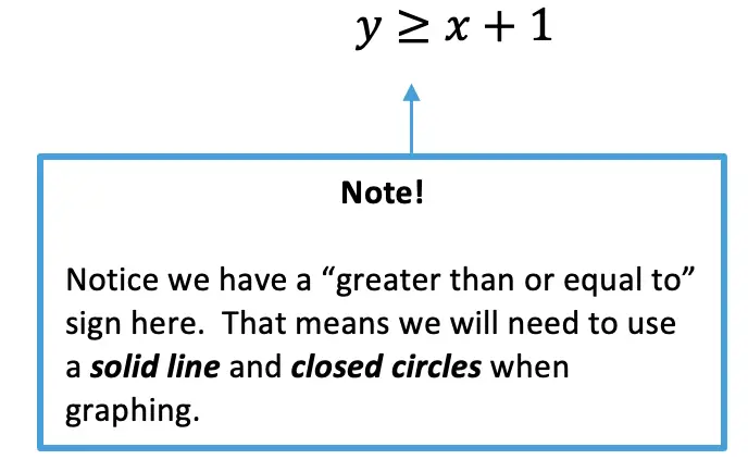
Step 6: Before graphing, let’s now identify what type of inequality we have here. Since we are working with a > sign, we will need to use a solid line and closed circles when creating our graph.
Step 7: Now that we have identified all the information we need to, let’s graph the second inequality below:
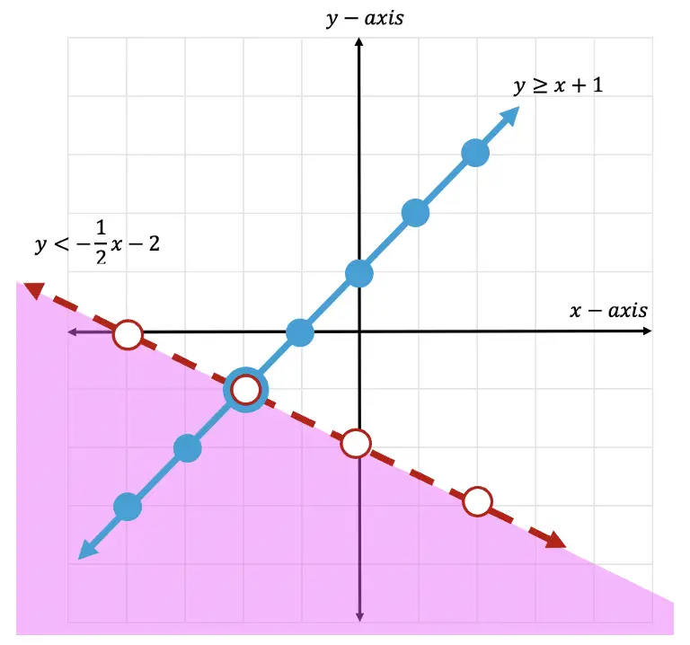
Step 8: Now it is time for us to shade our graph. Since we have a greater than or equal to sign, >, we will be shading above the x-axis. Notice all the positive y-values above are included to the left of our line. This is where we will shade.
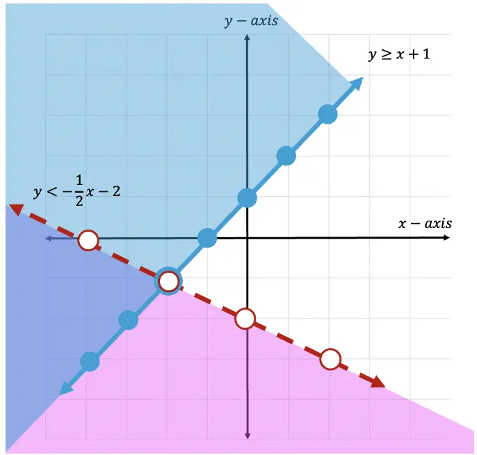
Where is the solution?!
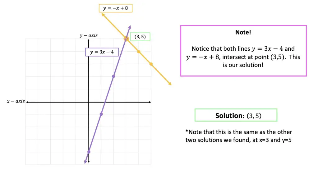
Step 9: The solution is found where the two shaded regions overlap. In this case, we can see that the two shaded regions overlap in the purple section of this graph.
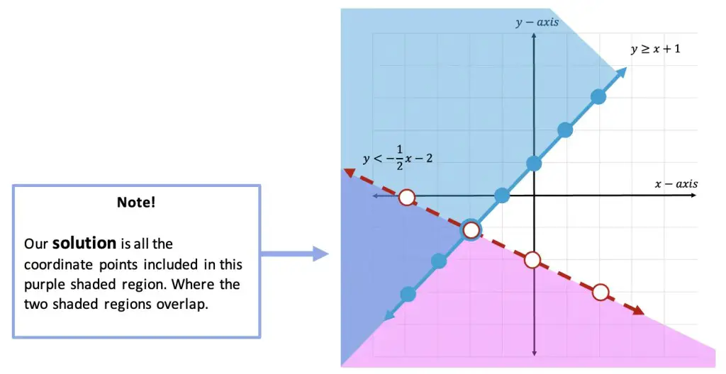
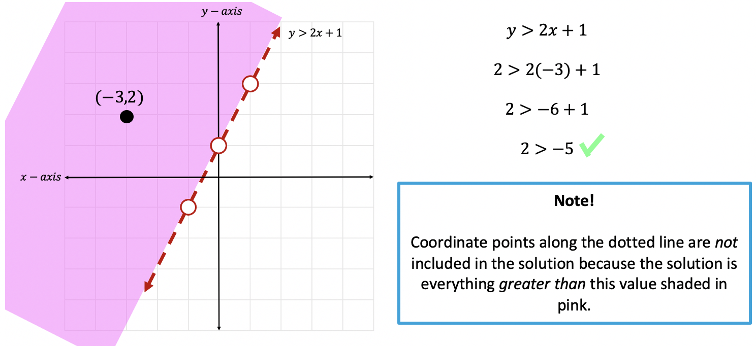
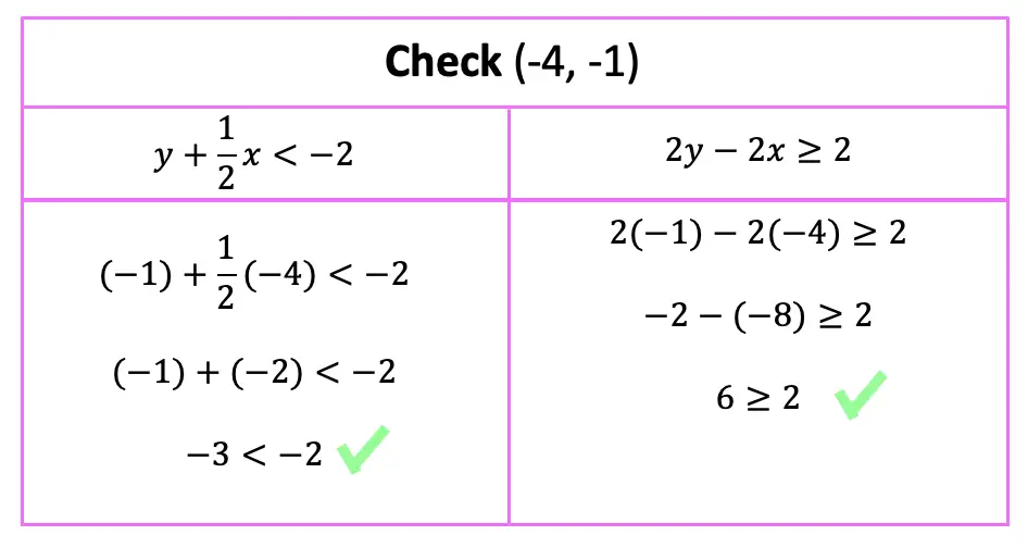
Step 10: Check! Now we can finally check our work. To do that, we can choose any point within our overlapping purple shaded region, if the coordinate point we choose holds true when plugged into both of our inequalities then our graph is correct!
Let’s take the point (-4,-1) and plug it into both original inequalities where x=-4 and y=-1.
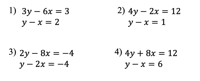
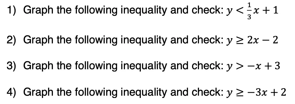
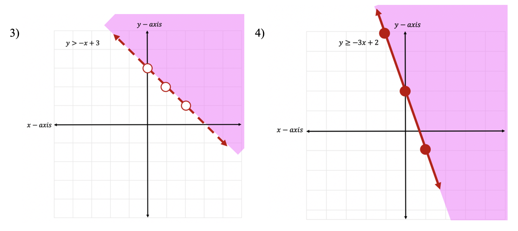
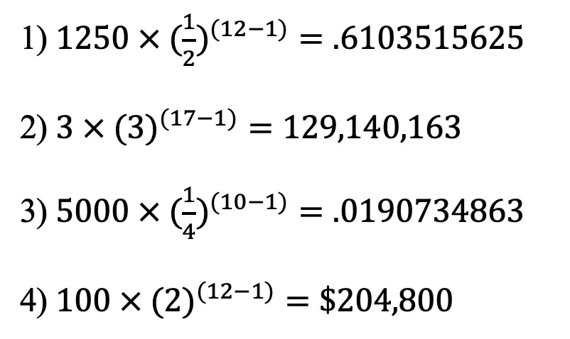
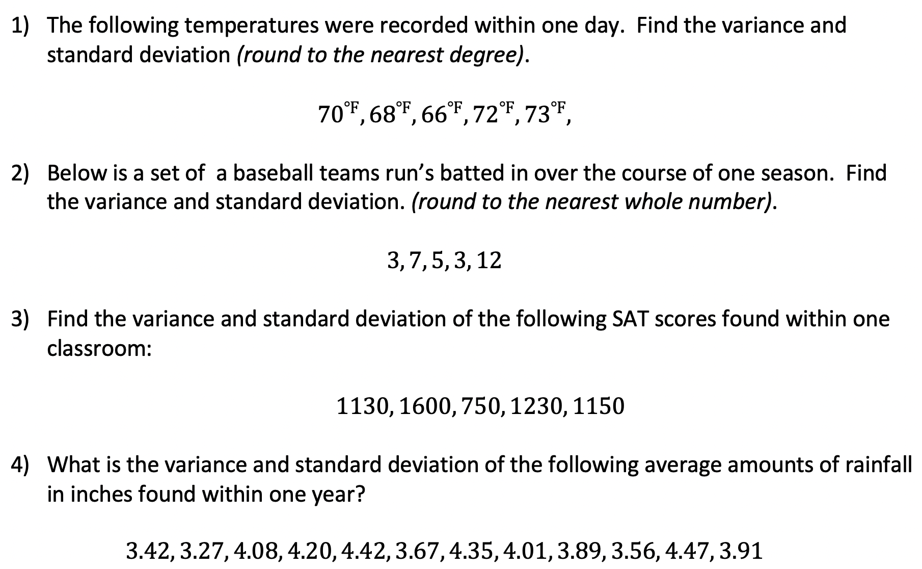
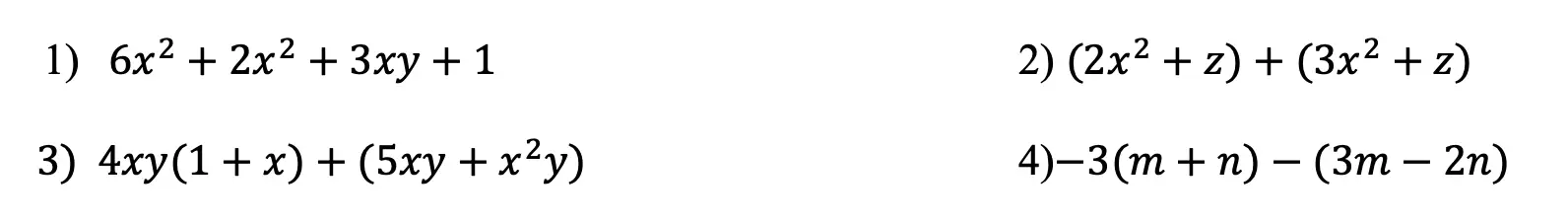
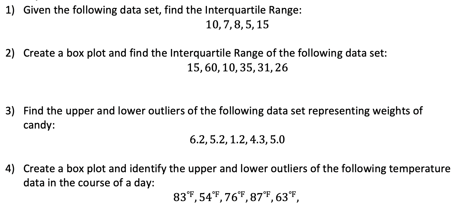
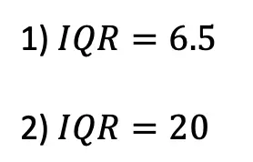
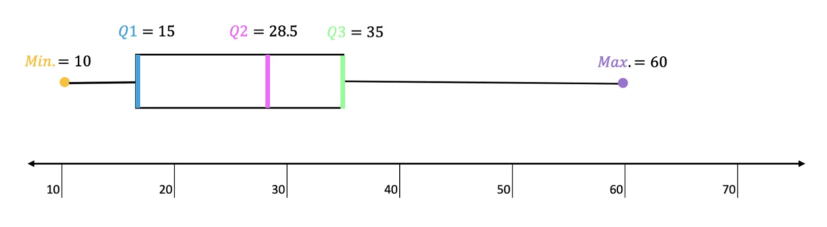
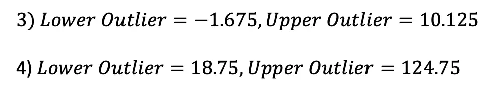
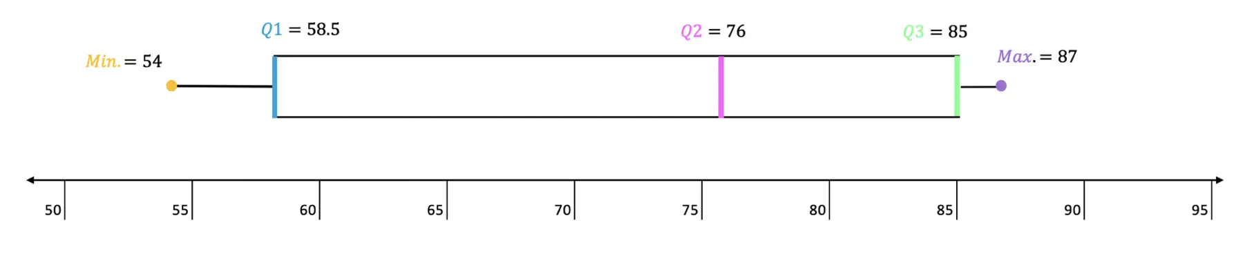
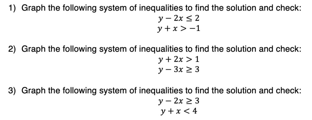
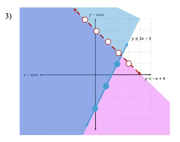
Practice Questions:
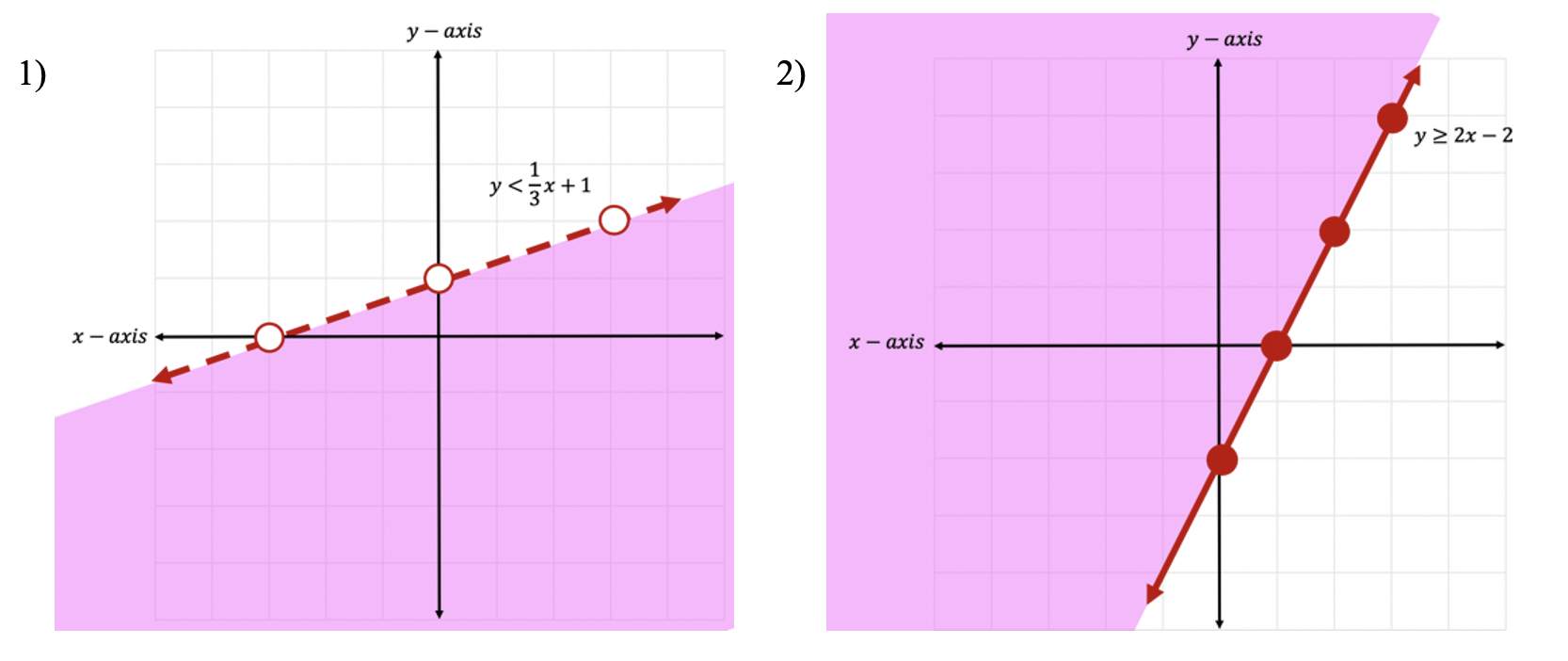
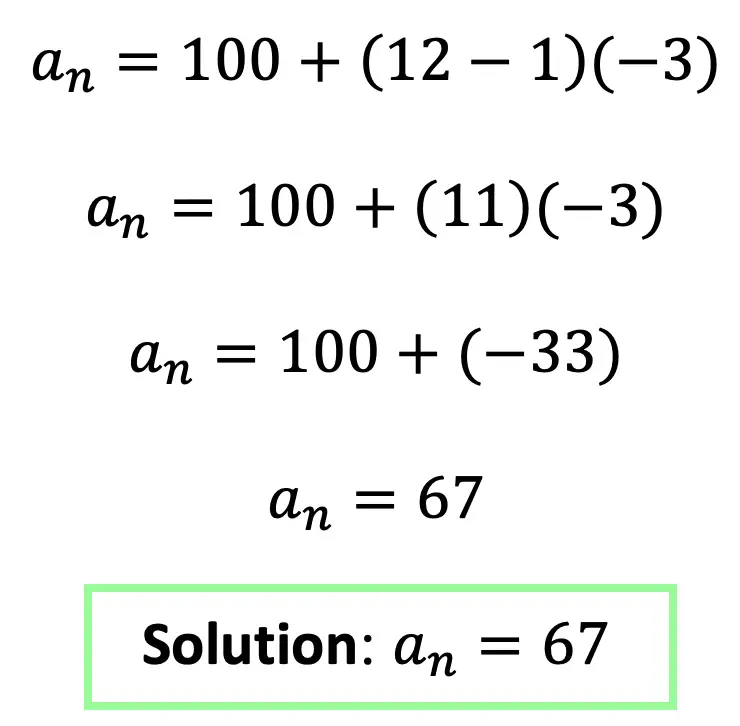
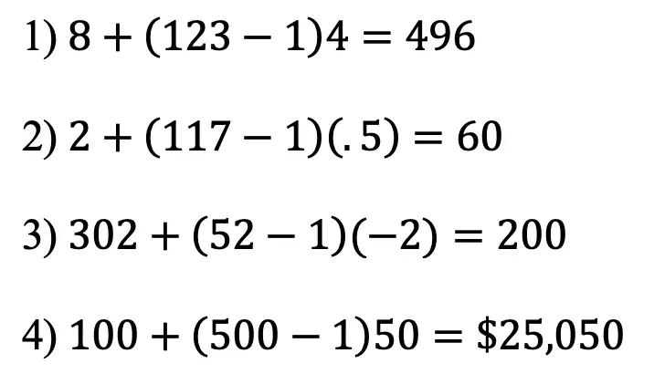
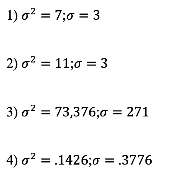
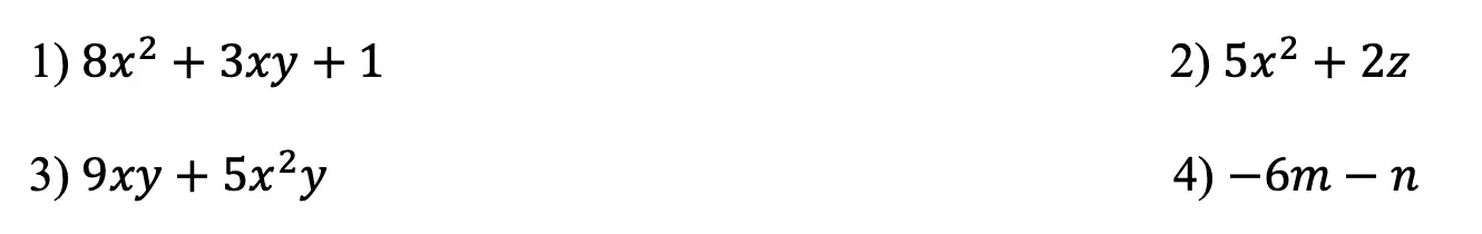
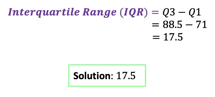
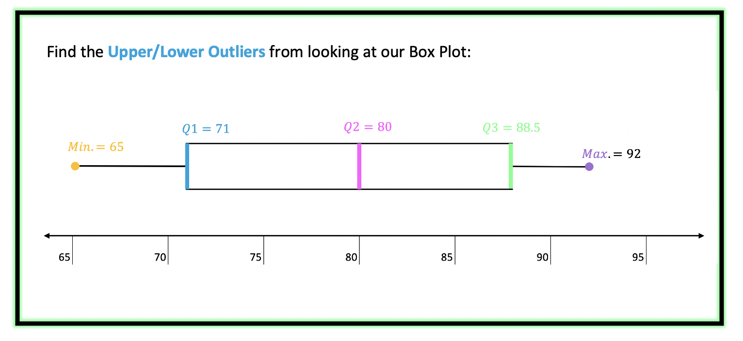
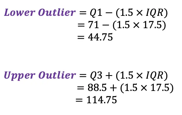
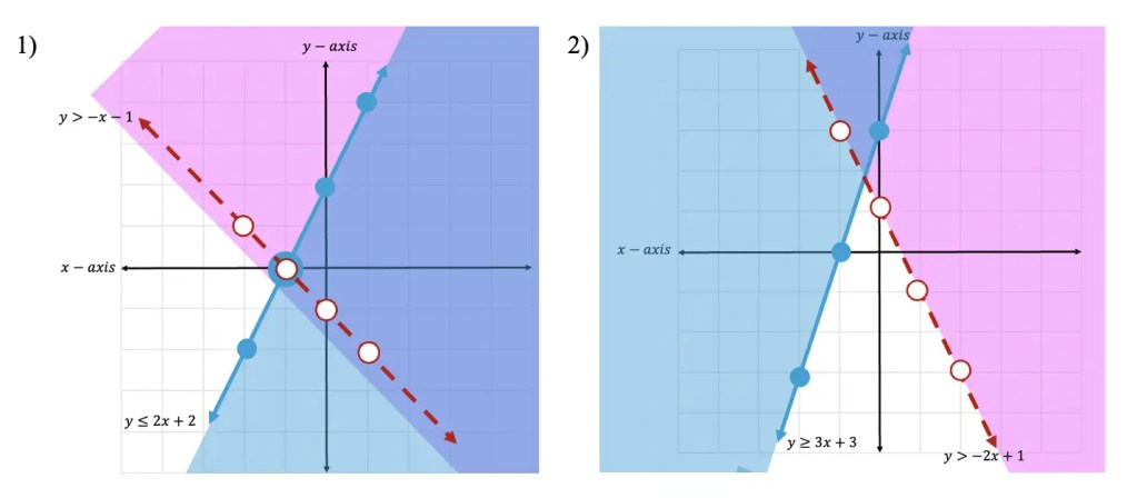
Solutions:
Still got questions? No problem! Don’t hesitate to comment with any questions below. Thanks for stopping by and happy calculating! 🙂
Facebook ~ Twitter ~ TikTok ~ Youtube
Looking to review graphing linear inequalities Check out this post on here!