How to Solve Inequalities with 2 Variables: Algebra

Hi everyone and happy Wednesday! Today we are going to look at how to solve inequalities with 2 variables. You may hear this in your class as “Simultaneous Inequalities” or “Systems of Inequalities,” all of these mean the same exact thing! The key to answering these types of questions, is to know how to graph inequalities and to know that the solution is always found where the two shaded regions overlap each other on the graph. We’re going to go over an example one step at time, then there will be practice questions at the end of this post that you can try on your own. Happy calculating! 🙂

How to Solve Inequalities with 2 Variables:

Just to review, when graphing linear inequalities, remember, we always want to treat the inequality as an equation of a line in  form….with a few exceptions:

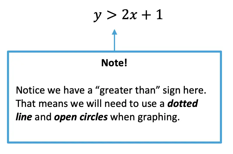
1)Depending on what type of inequality sign we are graphing, we will use either a dotted line and an open circle (< and >) or a solid line and a closed circle (> or <) and  to correctly represent the solution.

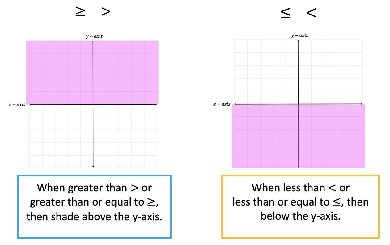
2) Shading is another important feature of graphing inequalities.  Depending on the inequality sign we will need to either shade above the x-axis ( > or > ) or below the x-axis ( < or < ) to correctly represent the solution.
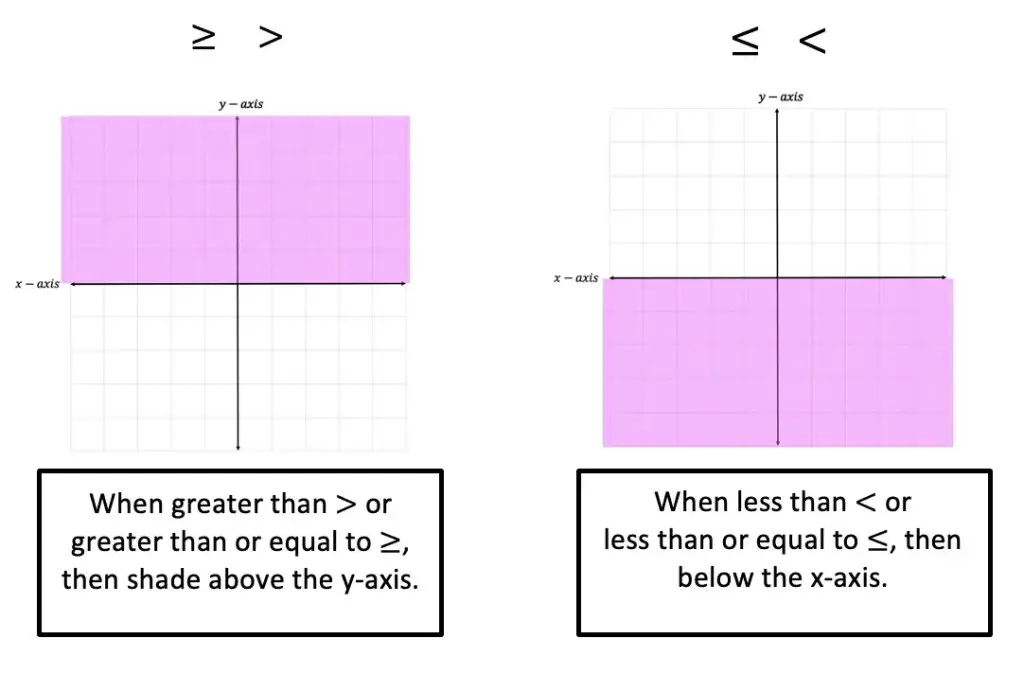
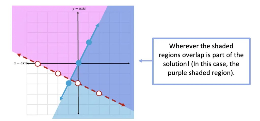
3) Solution: To find the solution of a system of inequalities, we are always going to look for where the shaded regions of both inequalities overlap.
How to Solve Inequalities with 2 Variables

Now that we know the rules, of graphing simultaneous inequalities, let’s take a look at an Example!

How to Solve Inequalities with 2 Variables

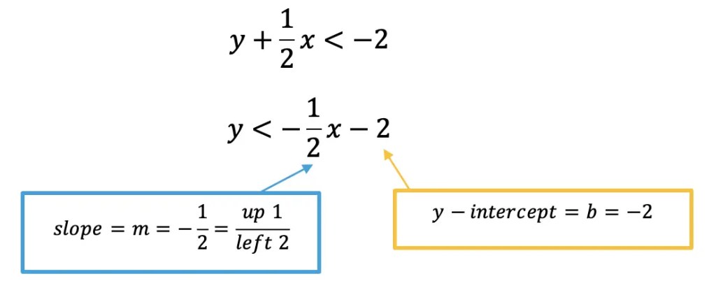
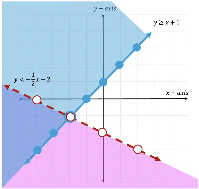
Step 1: First, let’s take our first inequality, and get it into y=mx+b form. To do this, we need to move .5x to the other side of the inequality by subtracting it from both sides. Once we do that, we can identify the slope and the y-intercept.
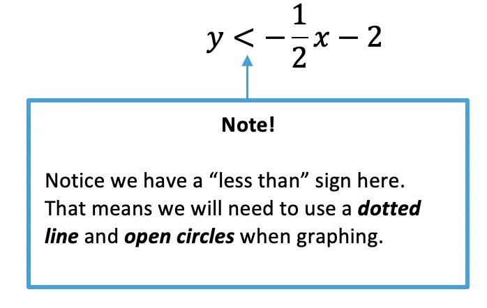
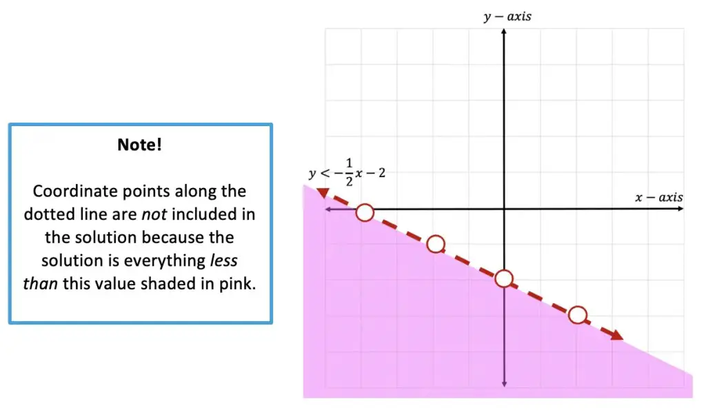
Step 2: Before graphing, let’s now identify what type of inequality we have here.  Since we are working with a < sign, we will need to use a dotted line and open circles when graphing.
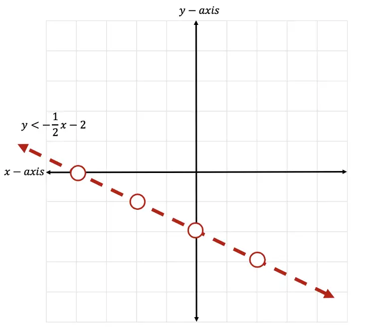
Step 3: Now that we have identified all the information we need to, let’s graph the first inequality below:
Step 4: Now it is time for us to shade our graph, since this is an inequality, we need to show all of our potential solutions with shading.  Since we have a less than sign, <, we will be shading below the x-axis.  Notice all the negative y-values below are included to the left of our line.  This is where we will shade.
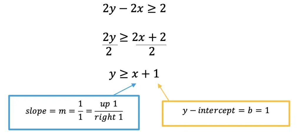
Step 5: Next, let’s start graphing our second inequality! We do this by taking the second equation, and getting it into y=mx+b form. To do this, we need to move 2x to the other side of the inequality by adding it to both sides. Then we can simplify the inequality even further by dividing out a 2.
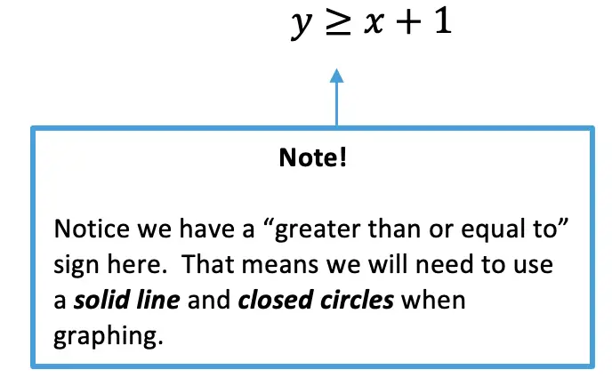
Step 6: Before graphing, let’s now identify what type of inequality we have here.  Since we are working with a > sign, we will need to use a solid line and closed circles when creating our graph.
Step 7: Now that we have identified all the information we need to, let’s graph the second inequality below:
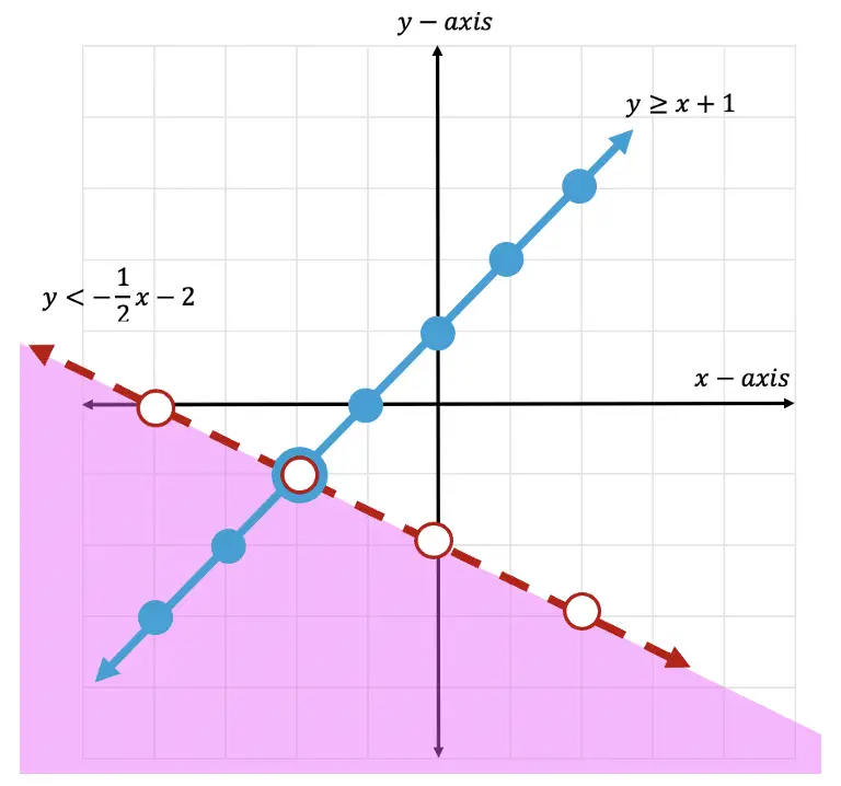
Step 8: Now it is time for us to shade our graph.  Since we have a greater than or equal to sign, >, we will be shading above the x-axis.  Notice all the positive y-values above are included to the left of our line.  This is where we will shade.
How to Solve Inequalities with 2 Variables

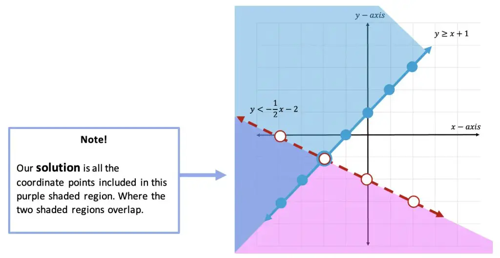
Where is the solution?!

Step 9: The solution is found where the two shaded regions overlap. In this case, we can see that the two shaded regions overlap in the purple section of this graph.
How to Solve Inequalities with 2 Variables

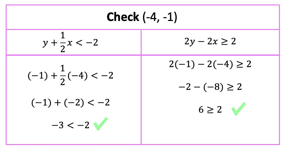
Step 10: Check!  Now we can finally check our work.  To do that, we can choose any point within our overlapping purple shaded region, if the coordinate point we choose holds true when plugged into both of our inequalities then our graph is correct!

Let’s take the point (-4,-1) and plug it into both original inequalities where x=-4 and y=-1.
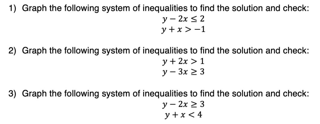
Practice Questions:
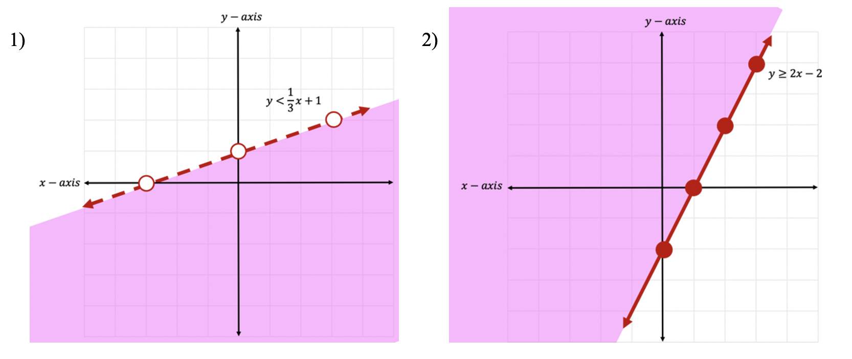
Solutions:
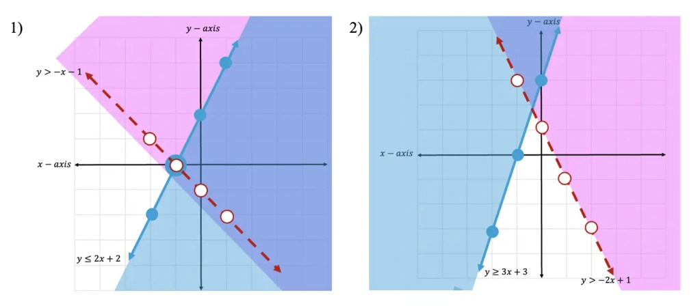
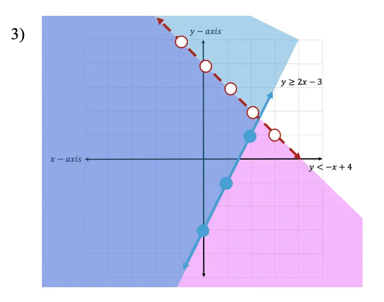
How to Solve Inequalities with 2 Variables

Still got questions? No problem! Don’t hesitate to comment with any questions below. Thanks for stopping by and happy calculating! 🙂

Facebook ~ Twitter ~ TikTok ~ Youtube

Looking to review graphing linear inequalities Check out this post on here!

Continuously Compounding Interest Formula

A=Pert

P=Principal (Original $ Amount Invested)

e=Mathematical Constant

r=Interest Rate

t=Time

Hi everyone and welcome to MathSux! In this post, we are going to go over the continuously compounding interest formula, A=Pert! This is a great topic as it relates to finance and real-world money situations (sort of). We are going to break down everything step by step by understanding what the continuously compounding interest rate formula A=Pert is, identifying each component of the formula, and then applying it to an example. If you’re looking for more, don’t forget to check out the video and the practice questions at the end of this post. Happy calculating! 🙂

What is Continuous Compounding Interest Formula?

Let’s say we have $500 and we want to invest it.

What if it compounded interest once a year? 

Twice a year? 

Once a day, or 365 days a year?

What if we compounded interest every second of the day for a total of 86,400 seconds throughout the year!?

And what if we kept going, making the number of times compounded annually more and more often to occur every half second? This is what Continuous Compounding Interest is, and it tells us how much we earn on a principle (original amount) if the compound interest rate for the year were to be granted an infinite number of times.

The weird thing is that continuous compounding interest is technically impossible (I’ve yet to see a bank that offers an infinite number of compounding interest!).  Even though it is impossible, in math and finance, we look at continuous compounding interest for theoretical purposes, in other words, it’s for money nerds! Luckily, it comes with an easy-to-use formula, let’s take a look:

Continuously Compounding Interest Formula

Now, let’s see this formula in action with the following Example:

Step 1: First, let’s write out our formula and identify what each value represents based on the question.

Continuously Compounding Interest Formula

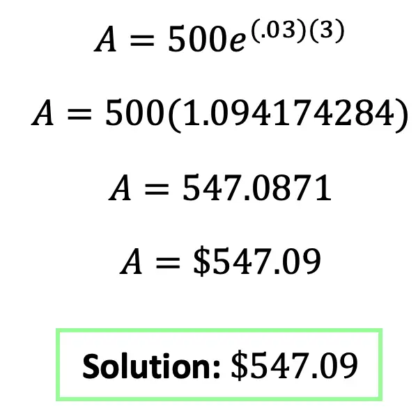
Step 2: Fill in our formula with the given values and solve.

Practice Questions:

1) Sally invested $1000 which was then continuously compounded by 4%. How much money will Sally have after 5 years?

2) Brad invested $1500 into an account continuously compounded by 5%. How much money will he have after 7 years?

3) Fran invests $2000 into an account that is continuously compounded by 1%. How much money will Fran earn by year 5?

Solutions:

1) $1,221.40

2) $2,128.60

3) $2,102.54

Want to make math suck just a little bit less? Subscribe to my Youtube channel for free math videos every week! 🙂

Facebook ~ Twitter ~ TikTok ~ Youtube

Looking to review more topics in Algebra? Check our Algebra page here!

Simultaneous Equations: Algebra

Happy new year and welcome to Math Sux! In this post we are going to dive right into simultaneous equations and how to solve them three different ways! We will go over how to solve simultaneous equations using the (1) Substitution Method (2) Elimination Method and (3) Graphing Method. Each and every method leading us to the same exact answer! At the end of this post don’t forget to try the practice questions choosing the method that best works for you! Happy calculating! 🙂

What are Simultaneous Equations?

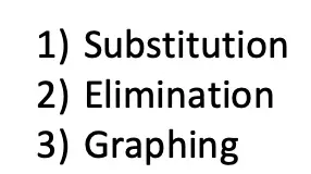
Simultaneous Equations are when two equations are graphed on a coordinate plane and they intersect at, at least one point.  The coordinate point of intersection for both equation is the answer we are trying to find when solving for simultaneous equations. There are three different methods for finding this answer:

We’re going to go over each method for solving simultaneous equations step by step with the example below:

Method #1: Substitution

The idea behind Substitution, is to solve for 1 variable first algebraically, and the plug this value back into the other equation solving for one variable.  Then solving for the remaining variable.  If this sounds confusing, don’t worry! We’re going to do this step by step:

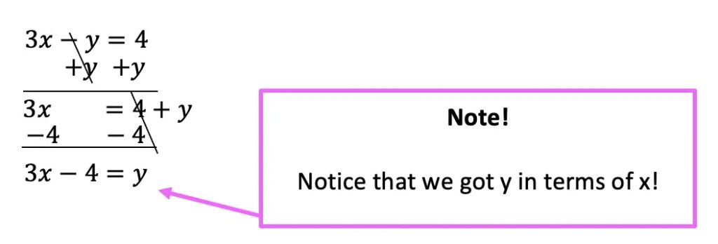
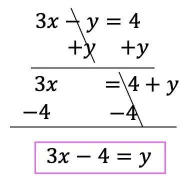
Step 1: Let’s choose the first equation and move our terms around to solve for y.

Simultaneous Equations

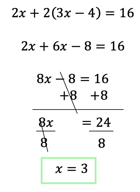
Step 3: The equation is set up and ready to solve for x!

Simultaneous Equations

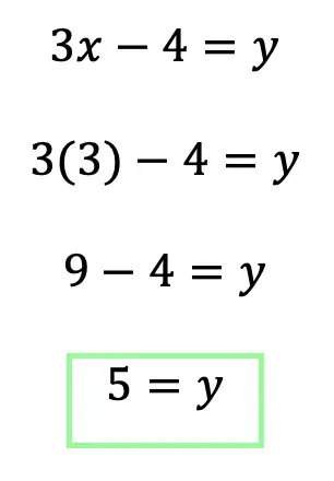
Step 4: All we need to do now, is plug x=3 into one of our original equations to solve for y.

Simultaneous Equations

Step 5: Now that we have solved for both x and y, we have officially found where these two simultaneous equations meet!

Simultaneous Equations

Method #2: Elimination

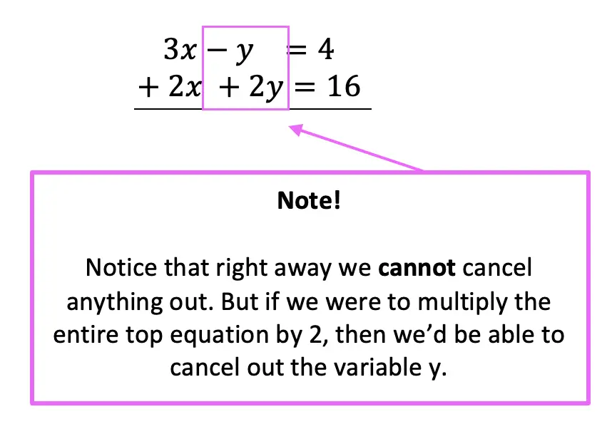
The main idea of Elimination is to add our two equations together to cancel out one of the variables, allowing us to solve for the remaining variable.  We do this by lining up both equations one on top of the other and adding them together.  If variables at first do not easily cancel out, we then multiply one of the equations by a number so it can. Check out how it’s done step by step below!

Step 1: First, let’s stack both equations one on top of the other to see if we can cancel anything out:

Simultaneous Equations

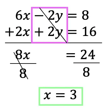
Step 2: Our goal is to get a 2 in front of y in the first equation, so we are going to multiply the entire first equation by 2.

Simultaneous Equations

Step 3: Now that we multiplied the entire first equation by 2, we can line up our two equations again, adding them together, this time canceling out the variable y to solve for x.

Simultaneous Equations

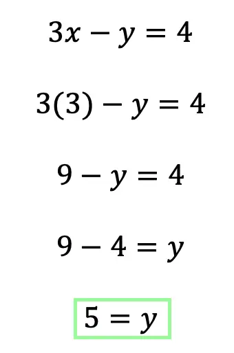
Step 4: Now, that we’ve found the value of variable x=3, we can plug this into one of our equations and solve for missing unknown variable y.

Simultaneous Equations

Step 5: Now that we have solved for both x and y, we have officially found where these two simultaneous equations meet!

This image has an empty alt attribute; its file name is Screen-Shot-2020-12-30-at-10.21.46-AM.png

Method #3: Graphing

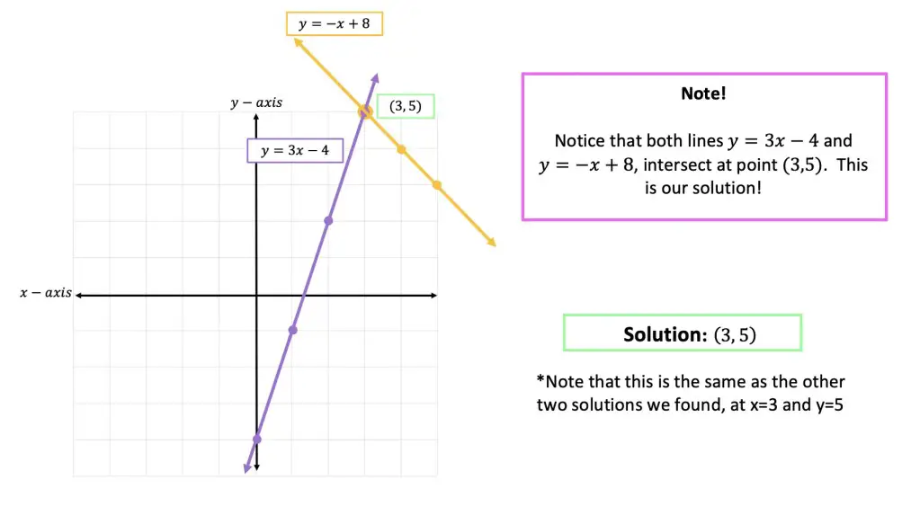
The main idea of Graphing is to graph each a equation on a coordinate plane and then see at what point they intersect.  This is the best method to visualize and check our answer!

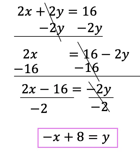
Step 1: Before we start graphing let’s convert each equation into y=mx+b (equation of a line) form.

Equation 1:

Equation 2:

Step 2: Now, let’s graph each line, y=3x-4 and y=-x+8, to see at what coordinate point they intersect.

Simultaneous Equations

Need to review how to draw an equation of a line? Check out this post here! Notice we got the same exact answer using all three methods (1) Substitution (2) Elimination and (3) Graphing.

Ready to try the practice problems on your own?! Check them out below!

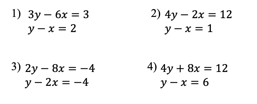
Practice Questions:

Solve the following simultaneous equations for x and y.

Solutions:

  1. (1, 3)
  2. (4,5)
  3. (-1, -6)
  4. (3, -3)

Want more MathSux?  Don’t forget to check out our Youtube channel and more below! And if you have any questions, please don’t hesitate to comment below. Happy Calculating!

Facebook ~ Twitter ~ TikTok ~ Youtube

If you are looking for a challenge, try solving three equations with three unknown variables, in this post here!

Graphing Linear Inequalities: Algebra

graphing linear inequalities

Hi and welcome to MathSux! In this post, we are going to go over the rules for graphing linear inequalities on a coordinate plane when it comes to drawing lines, circles , and shading, then we are going to solve an example step by step. If you have any questions, check out the video below and try the practice questions at the end of this post! If you still have questions, don’t hesitate to comment below and happy calculating! 🙂

Graphing Linear Inequalities:

When graphing linear inequalities, we always want to treat the inequality as an equation of a line in  form y=mx+b….with a few exceptions:

Graphing Linear Inequalities
inequality shading above or below y-axis

Now that we know the rules, of graphing inequalities, let’s take a look at an Example!

Graphing Linear Inequalities Example:

graphing inequality example

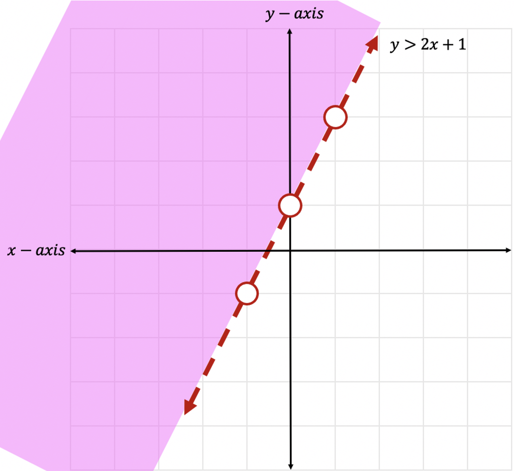
Step 1: First, let’s identify what type of inequality we have here.  Since we are working with a > sign, we will need to use a dotted line and open circles when creating our graph.

graphing inequality example

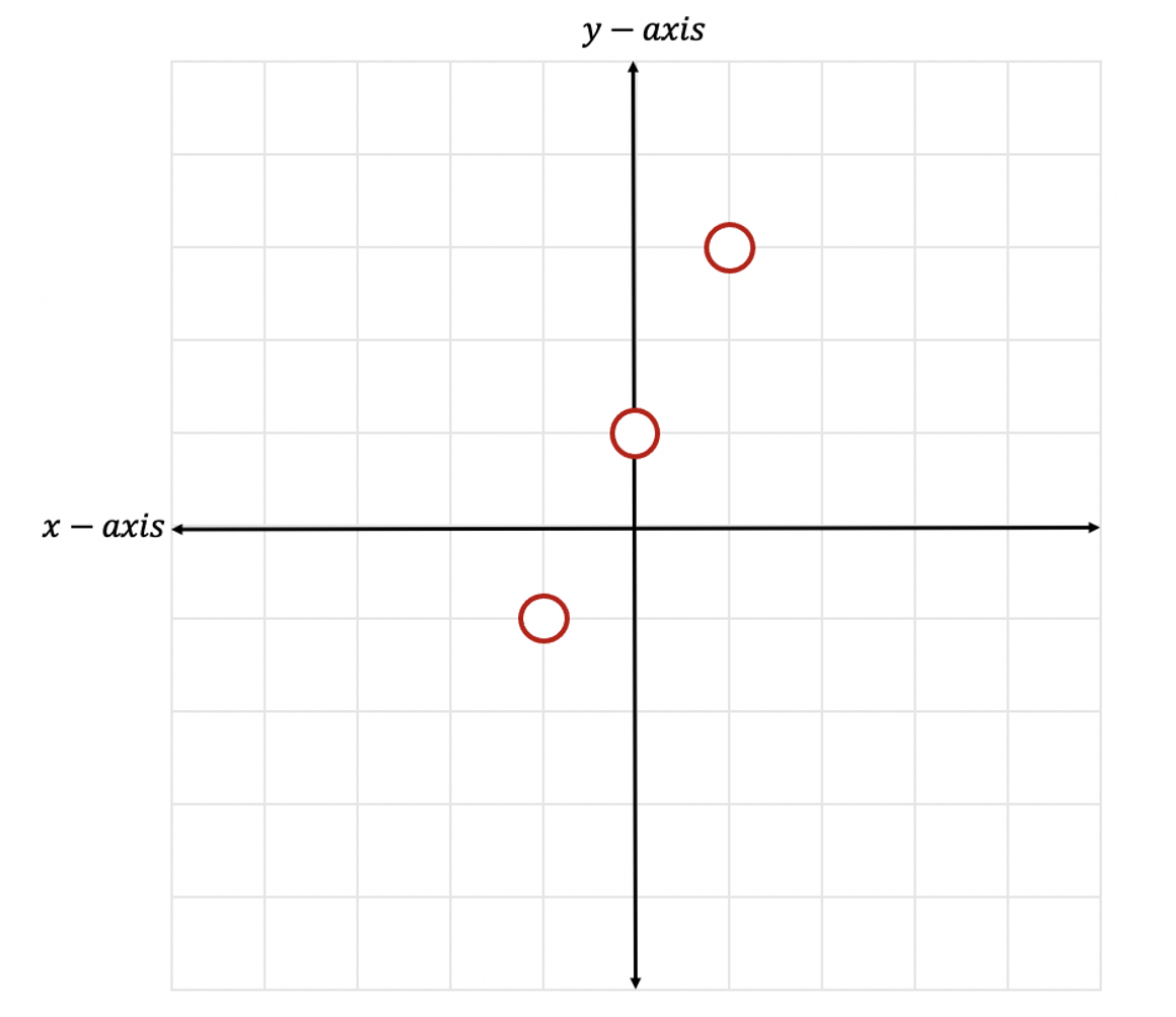
Step 2: Now we are going to start graphing our linear inequality as a normal equation of a line, by identifying the slope and the y-intercept only this time keeping open circles in mind.  (For a review on how to graph regular equation of a line in y=mx+b form, click here)

graphing inequality example
graphing linear inequalities

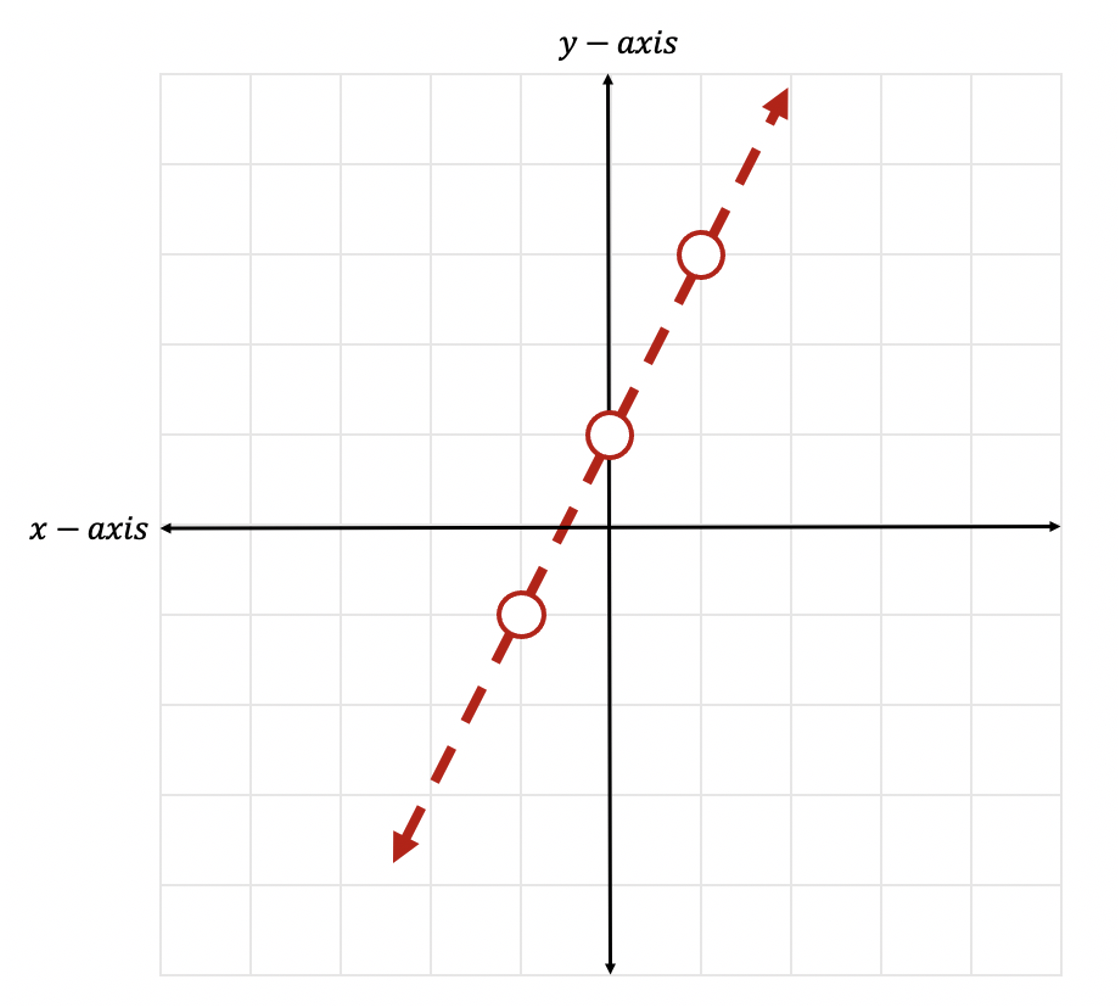
Step 3: Now let’s connect our dots, by using a dotted line to represent our greater than sign.

graphing linear inequalities

Step 4: Now it is time for us to shade our graph, since this is an inequality, we need to show all of our potential solutions with shading.  Since we have a greater than sign, , we will be shading above the y-axis.  Notice all the positive y-values above are included to the left of our line.  This is where we will shade.

graphing linear inequalities

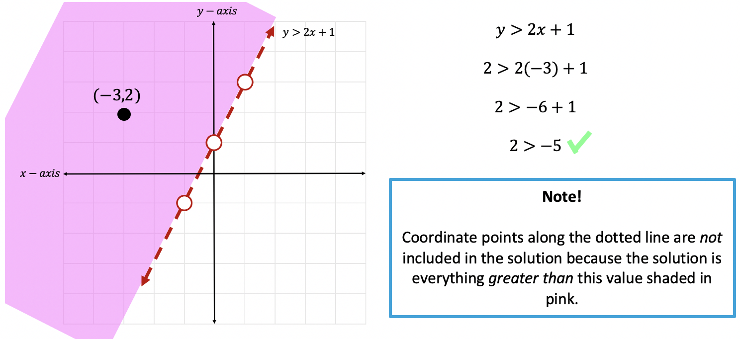
Step 5: Check!  Now we need to check our work.  To do that, we can choose any point within our shaded region, if the coordinate point we chose hold true when plugged into our inequality then we are correct!

Let’s take the point (-3,2) plugging it into our inequality where x=-3 and y=2.

graphing linear inequalities

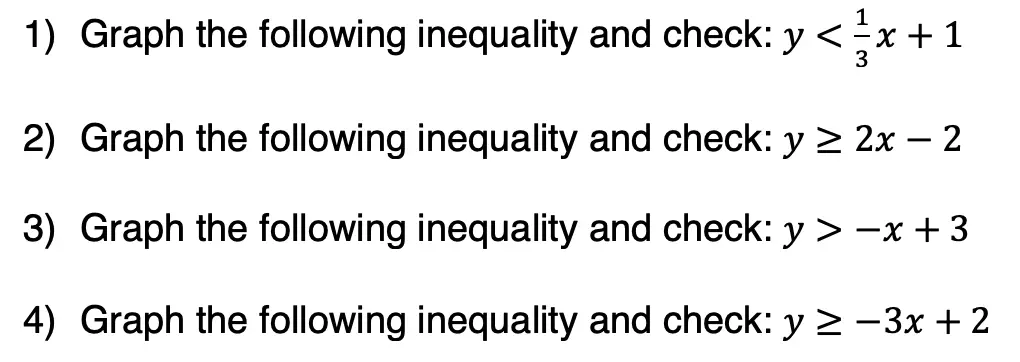
Practice Questions:

graphing linear inequalities

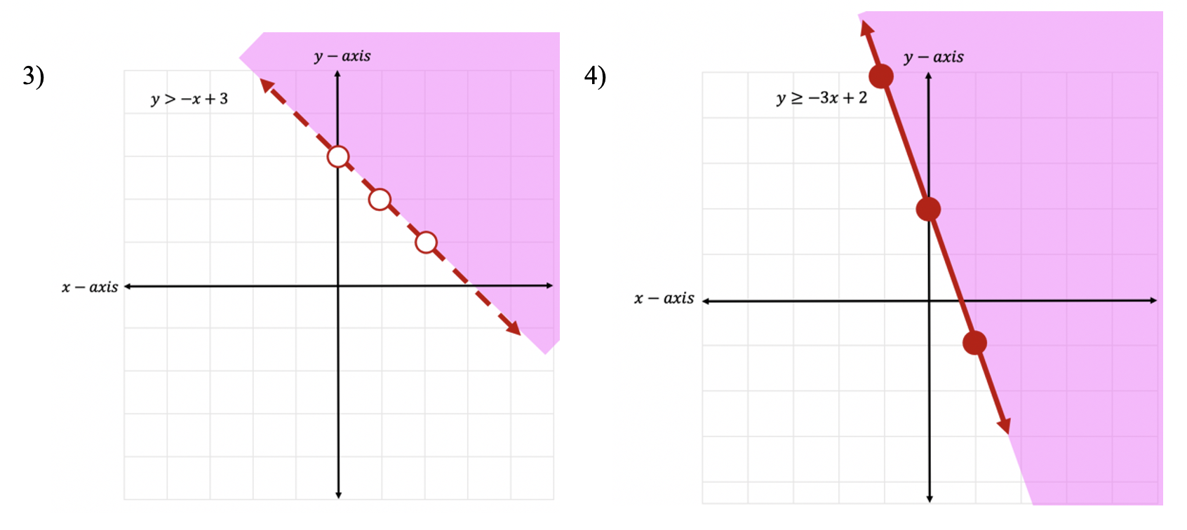
Solutions:

graphing linear inequalities

Still got questions? No problem! Don’t hesitate to comment with any questions or check out the video above for an in depth explanation. Happy calculating! 🙂

Facebook ~ Twitter ~ TikTok ~ Youtube

TikTok Math Video Compilations

Happy December everyone! With crazy 2020 coming to an end, I thought I would share some TikTok math video compilations of Algebra, Geometry, Algebra 2/Trig, and Statistics for a quick review of all our videos posted throughout the year. Enjoy these TikTok math video compilations and happy calculating! 🙂

Want to make math suck just a little bit less? Subscribe and follow us for FREE fun colorful math videos and lessons every week! 🙂

Facebook ~ Twitter ~ TikTok ~ Youtube

TikTok Math Video Compilations

Algebra:

Within algebra, you will find arithmetic sequences, combining like terms, box and whisker plots, geometric sequences, solving radical equations, completing the square, 4 ways to factor quadratic equations, piecewise functions and more!

Geometry:

Within Geometry, you will find, how to construct an equilateral triangle, a median of a trapezoid, area of a sector, how to find perpendicular and parallel lines through a given point, SOH CAH TOA right triangle trigonometry, reflections, and more!

Algebra 2/Trig.

Within Algebra 2/Trig., you will find, how to expand a cubed binomial, how to divide polynomials, how to solve log equations, imaginary numbers, synthetic division, unit circle basics, how to graph y=sin(x), and more!

Statistics:

Within statistics, you will find, box and whisker plots, how to find the variance, and, the probability of flipping a coin 2 times!

For full length video, don’t forget to check out our free math video index page! Thanks for stopping by! 🙂

What is a Geometric Sequence?

Geometric Sequence Formula:

an=a1r(n-1)

a1 = First Term

r=Common Ratio (Number Multiplied/Divided by each successive term in sequence)

n= Term Number in Sequence

Hi everyone and welcome to Mathsux! In this post, we are going to answer the question, what is a geometric sequence (otherwise known as a geometric progression)? We will accomplish this by learning how to identify a geometric sequence, then we will break down the geometric sequence formula an=a1r(n-1), and solve two different types of examples. As always if you want more questions, check out the video below and the practice problems at the end of this post. Happy calculating! 🙂

What are Geometric Sequences?

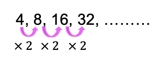
Geometric sequences are a sequence of numbers that form a pattern when the same number is either multiplied or divided to each subsequent term. Take a look at the example of a geometric sequence below:

Example:

geometric progression

Notice we are multiplying 2 by each term in the sequence above. If the pattern were to continue, the next term of the sequence above would be 64. This is a geometric sequence!

In this geometric sequence, it is easy for us to see what the next term is, but what if we wanted to know the 15th term?  Instead of writing out and multiplying our terms 15 times, we can use a shortcut, and that’s where the Geometric Sequence formula comes in handy!

Geometric Sequence Formula:

Take a look at the geometric sequence formula below, where each piece of our formula is identified with a purpose.

an=a1r(n-1)

a1 = The first term is always going to be that initial term that starts our geometric sequence. In this case, our sequence is 4,8,16,32, …… so our first term is the number 4.

r= One key thing to notice about the formula below that is unique to geometric sequences is something called the Common Ratio. The common ratio is the number that is multiplied or divided to each consecutive term within the sequence.

n= Another interesting piece of our formula is the letter n, this always stands for the term number we are trying to find. A great way to remember this is by thinking of the term we are trying to find as the nth term, which is unknown.

geometric sequences

Now that we broke down our geometric sequence formula, let’s try to answer our original question below:

Example #1: Common ratio r>1

Step 1: First let’s identify the common ratio between each previous and subsequent term of the sequence. Notice each term in the sequence is multiplied by 2 (as we identified earlier in this post). Therefore, our common ratio for this sequence is 2.

geometric progression

Step 2: Next, let’s write the geometric sequence formula and identify each part of our formula (First Term=4, Term number=15, common ratio=2).

geometric sequences

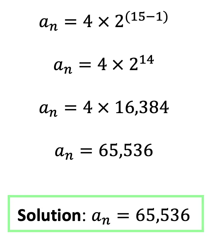
Step 3: Now let’s fill in our formula and solve with the given values.

geometric sequences

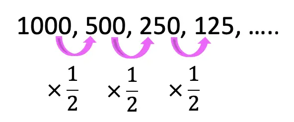
Let’s look at another example where, the common ratio is a bit different, and instead of multiplying a number, this time we are going to be dividing the same number from each subsequent term, (this can also be thought of as multiplying by a common ratio that is a fraction):

Example #2: Common ratio 0<r<1

Step 1: First let’s identify the common ratio between each number in the sequence. Notice each term in the sequence is divided by 2 (or multiplied by 1/2 that way it is shown below).

geometric progression

Step 2: Next, let’s write the geometric sequence formula and identify each part of our formula (First Term=1000, Term number=10, common ratio=1/2).

geometric sequences

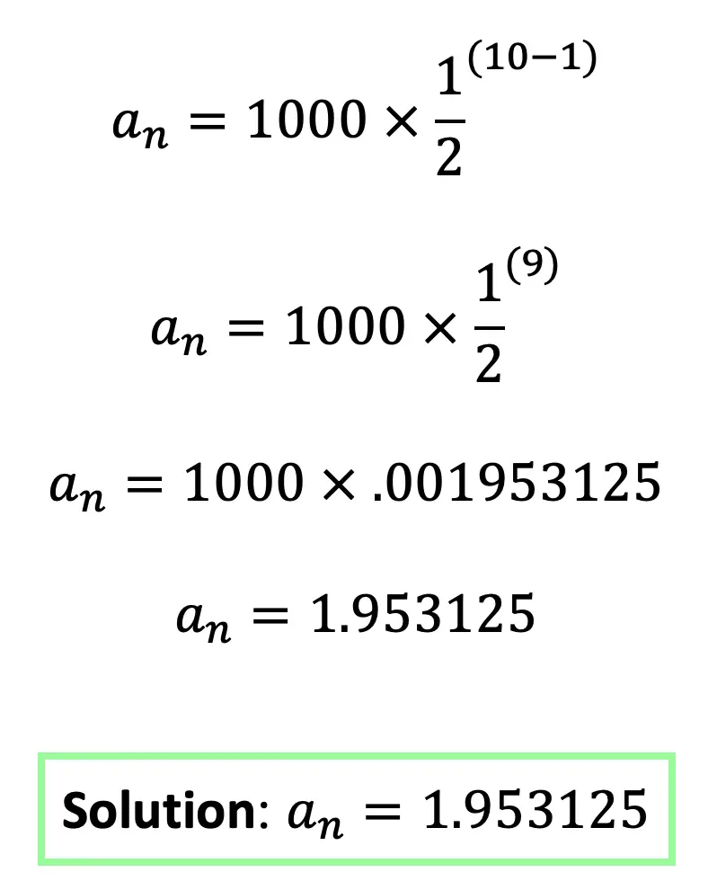
Step 3: Next let’s fill in our formula and solve with the given values.

Think you are ready to practice solving geometric sequences on your own? Try the following practice questions with solutions below:

Practice Questions:

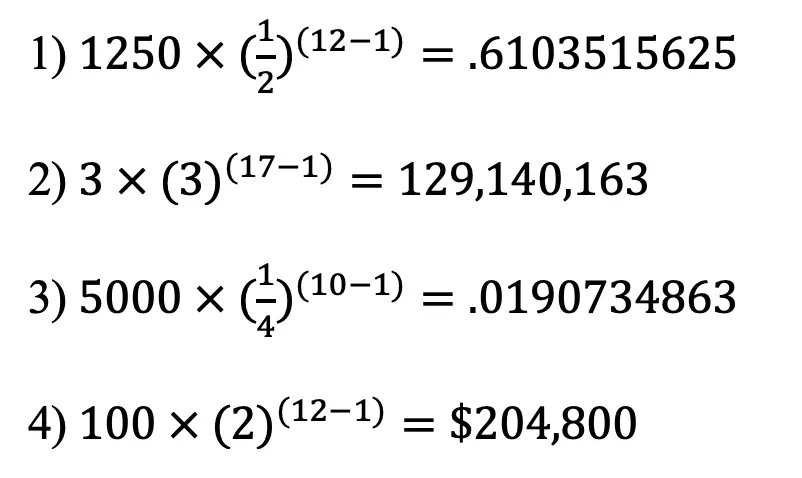
  1. Find the 12th term given the following sequence: 1250, 625, 312.5, 156.25, 78.125, ….
  2. Find the 17th term given the following sequence: 3, 9, 27, 81, 243,…..
  3. Find the 10th term given the geometric sequence: 5000, 1250, 312.5, 78.125 …..
  4. Shirley has $100 that she deposits in the bank. She continues to deposit twice the amount of money every month. How much money will she deposit in the twelfth month at the end of the year?

Solutions:

Fun Fact!

Did you know that the geometric sequence formula can be considered an explicit formula? An explicit formula means that even though we do not know the other terms of a sequence, we can still find the unknown value of any term within the given sequence. For example, in the first example we did in this post (example #1), we wanted to find the value of the 15th term of the sequence. We were able to do this by using the explicit geometric sequence formula, and most importantly, we were able to do this without finding the first 14 previous terms one by one…life is so much easier when there is an explicit geometric sequence formula in your life!

Other examples of explicit formulas can be found within the arithmetic sequence formula and the harmonic series.

Related Posts:

Looking to learn more about sequences? You’ve come to the right place! Check out these sequence resources and posts below. Personally, I recommend looking at the finite geometric sequence or infinite geometric series posts next!

Arithmetic Sequence

Recursive Formula

Finite Arithmetic Series

Finite Geometric Series

Infinite Geometric Series

Golden Ratio in the Real World

Fibonacci Sequence

Still, got questions? No problem! Don’t hesitate to comment below or reach out via email. And if you would like to see more MathSux content, please help support us by following ad subscribing to one of our platforms. Thanks so much for stopping by and happy calculating!

Facebook ~ Twitter ~ TikTok ~ Youtube

Arithmetic Sequence Formula:

an=a1+(n-1)d

a1=First Term

n=Term Number in Sequence

d=Common Difference (Number Added/Subtracted to each Term in Sequence)

Hi everyone and welcome to Mathsux! In this post, we’re going to go over arithmetic sequences (otherwise known as arithmetic progression). We’ll identify what arithmetic sequences are, break down each part of the arithmetic sequence formula an=a1+(n-1)d, and solve two different types of examples. As always if you want more questions, check out the video below and the practice problems at the end of this post. Happy calculating! 🙂

What are Arithmetic Sequences?

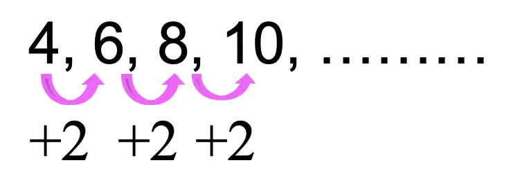
Arithmetic sequences are a sequence of numbers that form a pattern when the same number is either added or subtracted to each successive term. Take a look at the example of an arithmetic sequence below:

arithmetic sequences

Notice the pattern? We are adding the number 2 to each term in the sequence above. If the pattern were to continue, the next term of the sequence above would be 10+2 which gives us 12. This is an arithmetic sequence!

In the above sequence, it’s easy for us to identify what the next term in the sequence would be, but what happens if we were asked to find the 123rd term of an arithmetic sequence?  That’s where the Arithmetic Sequence Formula would come in handy!

Arithmetic Sequence Formula:

Take a look at the arithmetic sequence formula below, where each piece of our formula is identified with a purpose.

an=a1+(n-1)d

a1= The first term is always going to be that initial term that starts our arithmetic sequence. In this case, our sequence is 4,6,8,10, …… so our first term is the number 4.

n= Another interesting piece of our formula is the letter n, this always stands for the term number we are trying to find. A great way to remember this is by thinking of the term we are trying to find as the nth term, which is unknown.

d = One key thing to notice about the formula below that is unique to arithmetic sequences is something called the Common Difference. The common difference is the number that is added or subtracted to each consecutive term within the sequence.

explicit formula

Now that we know the arithmetic sequence formula, let’s try to answer our original question below:

arithmetic progression

Step 1: First let’s identify the common difference between each previous and subsequent term of the sequence. Notice each term in the sequence is being added by 2 (like we identified earlier in this post). Therefore, our common difference for this sequence is 2.

constant difference

Step 2: Next, let’s write the arithmetic sequence formula and identify each part of our formula (First Term=4, Term number=123, common difference=2).

arithmetic sequence formula

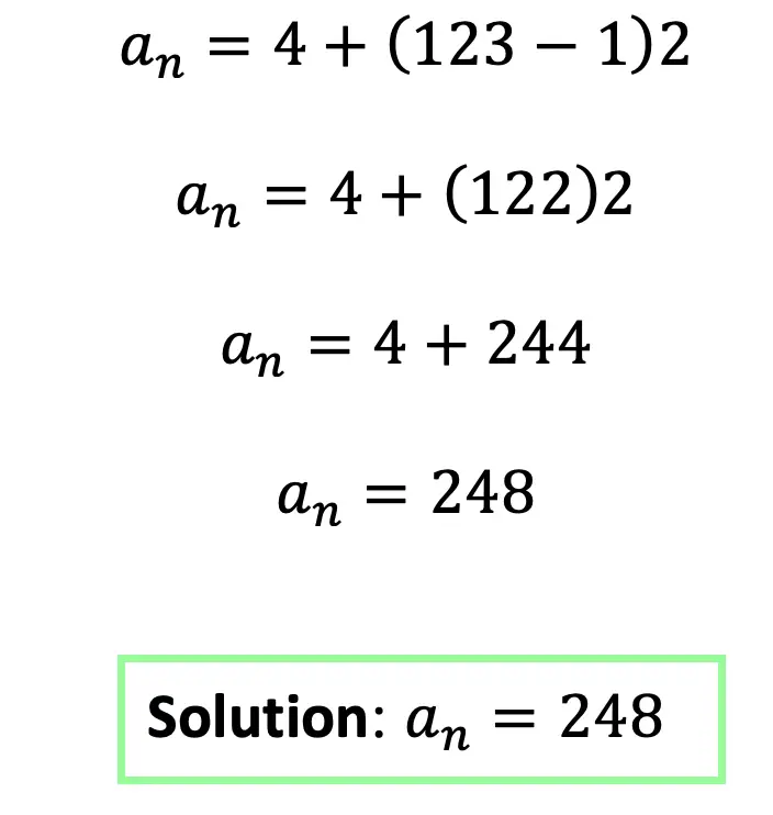
Step 3: Fill in our formula and solve with the given values.

math tutors

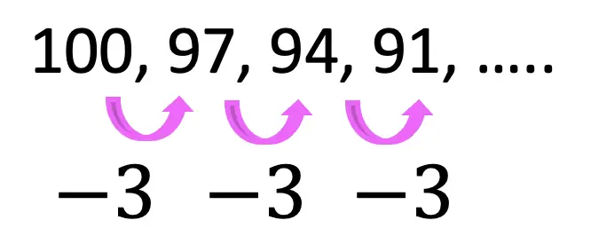
Now let’s look at another example where we subtract the same number from each term in the sequence, making the common difference negative.

arithmetic progression

Step 1: First let’s identify the common difference between each previous term and each subsequent term of the sequence. Notice each term in the sequence is being subtracted by 3. Therefore, our common difference for this sequence is -3, negative, because we are subtracting.

common difference

Step 2: Next, let’s write the arithmetic sequence formula and identify each part of our formula (First Term=100, Term number=12, common difference=-3).

arithmetic sequences

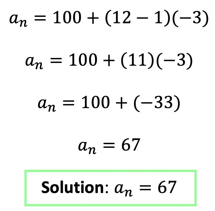
Step 3: Finally, let’s fill in our formula and solve with the given values.

Think you are ready to practice solving arithmetic sequences on your own? Try the following practice questions with solutions below:

Practice Questions:

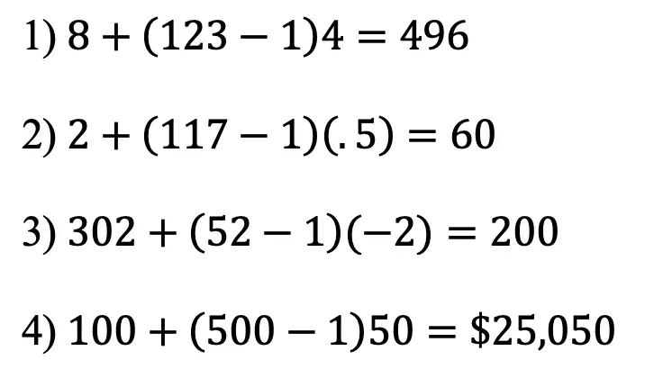
  1. Find the 123rd term given the following sequence: 8, 12, 16, 20, 24, ….
  2. Find the 117th term given the following sequence: 2, 2.5, 3, 3.5, …..
  3. Find the 52nd term given arithmetic sequence: 302, 300, 298, …..
  4. A software engineer charges $100 for the first hour of consulting and $50 for each additional hour.  How much would 500 hours of the consultation cost?

Solutions:

Still got questions? No problem! Don’t hesitate to comment with any questions or check out the video above. Happy calculating! 🙂

Fun Fact!

Did you know that the arithmetic sequence formula can be considered an explicit formula? An explicit formula means that even though we do not know the other terms of a sequence, we can still find the unknown value of any term within the given sequence. For example, in the first example we did in this post (example #1), we wanted to find the value of the 123rd term of the sequence. We were able to do this by using the explicit arithmetic sequence formula, and most importantly, we were able to do this without finding the first 122 previous terms one by one…life is so much easier when there is an explicit arithmetic sequence formula in your life!

Other examples of explicit formulas can be found within the geometric sequence formula and the harmonic series.

Related Posts:

Looking to learn more about sequences? You’ve come to the right place! Check out these sequence resources and posts below. Personally, I recommend looking at the geometric sequence or finite arithmetic series posts next!

Geometric Sequence

Recursive Formula

Finite Arithmetic Series

Finite Geometric Series

Infinite Geometric Series

Golden Ratio in the Real World

Fibonacci Sequence

Still, got questions? No problem! Don’t hesitate to comment below or reach out via email. And if you would like to see more MathSux content, please help support us by following ad subscribing to one of our platforms. Thanks so much for stopping by and happy calculating!

Facebook ~ Twitter ~ TikTok ~ Youtube

Variance and Standard Deviation: Statistics

Greetings math friends! In this post, we arere going to go over the formulas for Variance and Standard Deviation. We will take this step by step by explaining the significance of the variance and standard deviation formulas in relation to a set of data. Get your calculators ready because this step by step although not hard, will take some serious number crunching! Also, don’t forget to check out the video on standard deviation and variance below to see how to check your work using a calculator. Happy calculating! 🙂

If you’re looking for related formulas, Mean Absolute Deviation (MAD) and Expected Value, scroll to the bottom of this post! And if you’re interested we’ll also touch upon the difference between population variance and sample variance later in this post.

What is the Variance?

The variance represents the spread of data or the distance each data point is from the mean.  When we have multiple observations in our data, we want to know how far each unit of data is from the mean.  Are all the data points close together or spread far apart? What is the probability distribution? This is what the variance will help tell us!

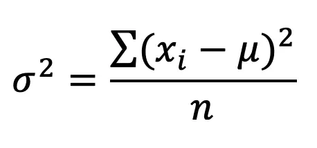
Don’t freak out but here’s the formula for variance, notated as using the greek letter, sigma squared, σ2:

Variance and Standard Deviation

where…

xi= Value of Data Point

μ= mean

n=Total Number of Data Points]

(xi-μ)=Distance each data point is to the mean

In plain English, this translates to:

variance formula

Let’s try an example to find the standard deviation and variance of the data set below.

variance formula
Variance and Standard Deviation

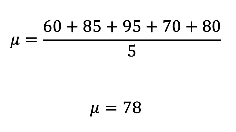
Step 1: First, let’s find the mean, μ.

Variance and Standard Deviation

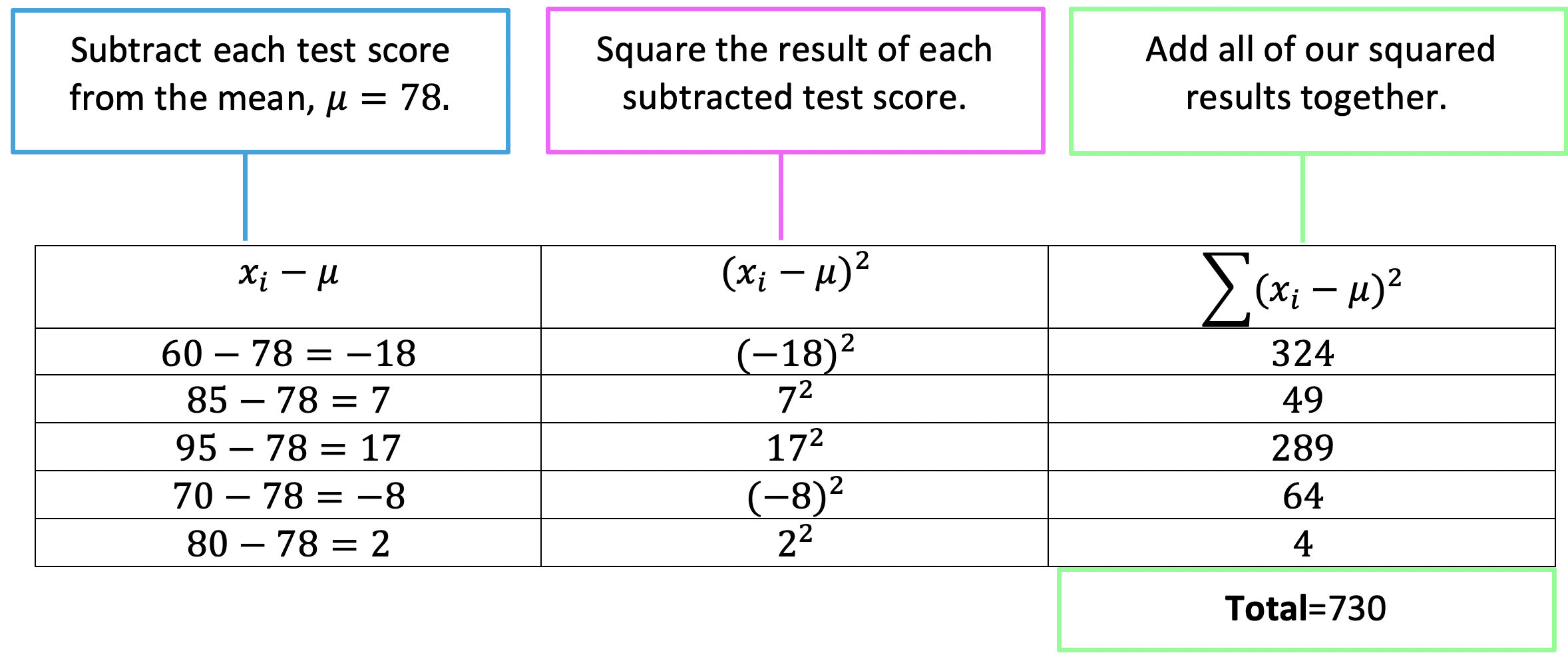
Step 2: Now that we have the mean, we are going to do each part of our formula one step at a time in the table below.

Notice we subtract each test score from the mean, μ=78. Then we square the result of each subtracted test score to get the squared deviation of each data value, then finally sum all the squared results together.

Variance and Standard Deviation

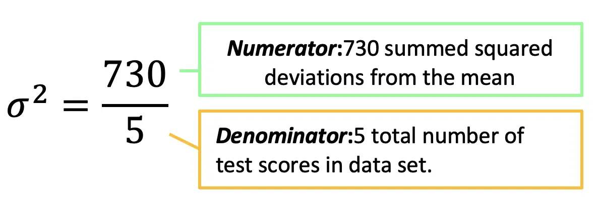
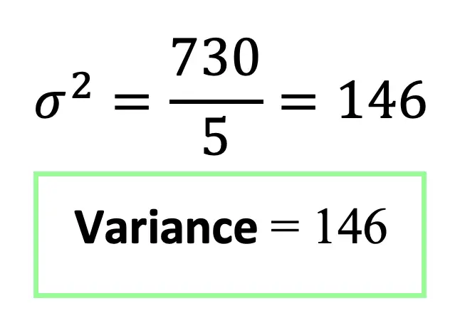
Step 3: Now that we summed all of our squared deviations, to get 730, we can fill this in as our numerator in the variance formula. We also know our denominator is equal to 5 because that is the total number of test scores in our data set.

Variance and Standard Deviation

What is Standard Deviation?

Standard deviation is a unit of measurement that is unique to each data set and is used to measure the spread of data. The standard deviation formula happens to be very similar to the variance formula!

Below is the formula for standard deviation, notated as sigma, the greek letter, σ:

sample standard deviation

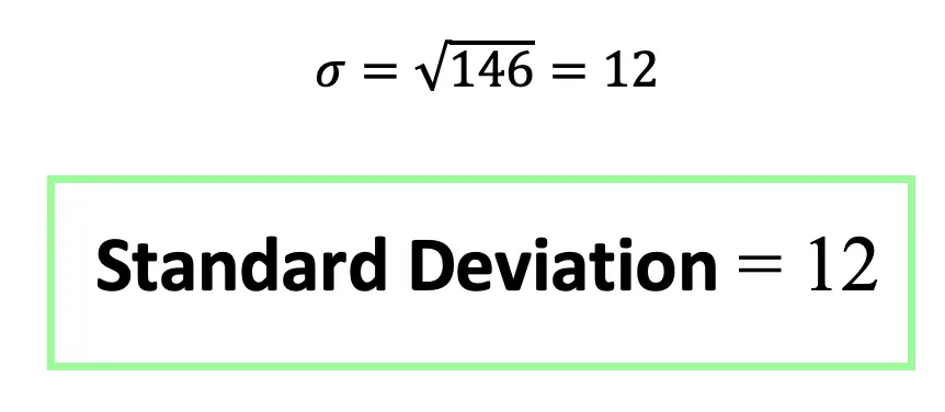
Since this is the same exact formula as variance with a square root, all we need to do is take the square root of the variance to find standard deviation:

sample standard deviation

Sample VS. Population

What is the difference between a sample vs. a population?

A population in statistics refers to an entire data set that at times can be humanly incapable of reaching.

For example: If we wanted to know the average income of everyone who lives in New York State, it would be almost impossible to reach every working person and ask them how much they make for a living.

To make up for the impossibility of data collection, we usually only survey a sample of the entire population to get income levels of let’s say 10,000 people across New York State, a much more reasonable in terms of data collecting!

And taking this sample size from the entire working population of New York State provides us with a sample mean, a sample variance, and a sample standard deviation.

On the other hand, if we were able to ask every student in a school what their grade point average was and get an answer, this would be an example of a whole population. Using this information, we would be able to find the population mean, population variance, and population standard deviation.

Sample notation also differs from population notation, but don’t worry about these too much, because the formulas and meanings remain the same. For example, the population mean is represented by the greek letter, μ, but the sample mean is represented by x bar.

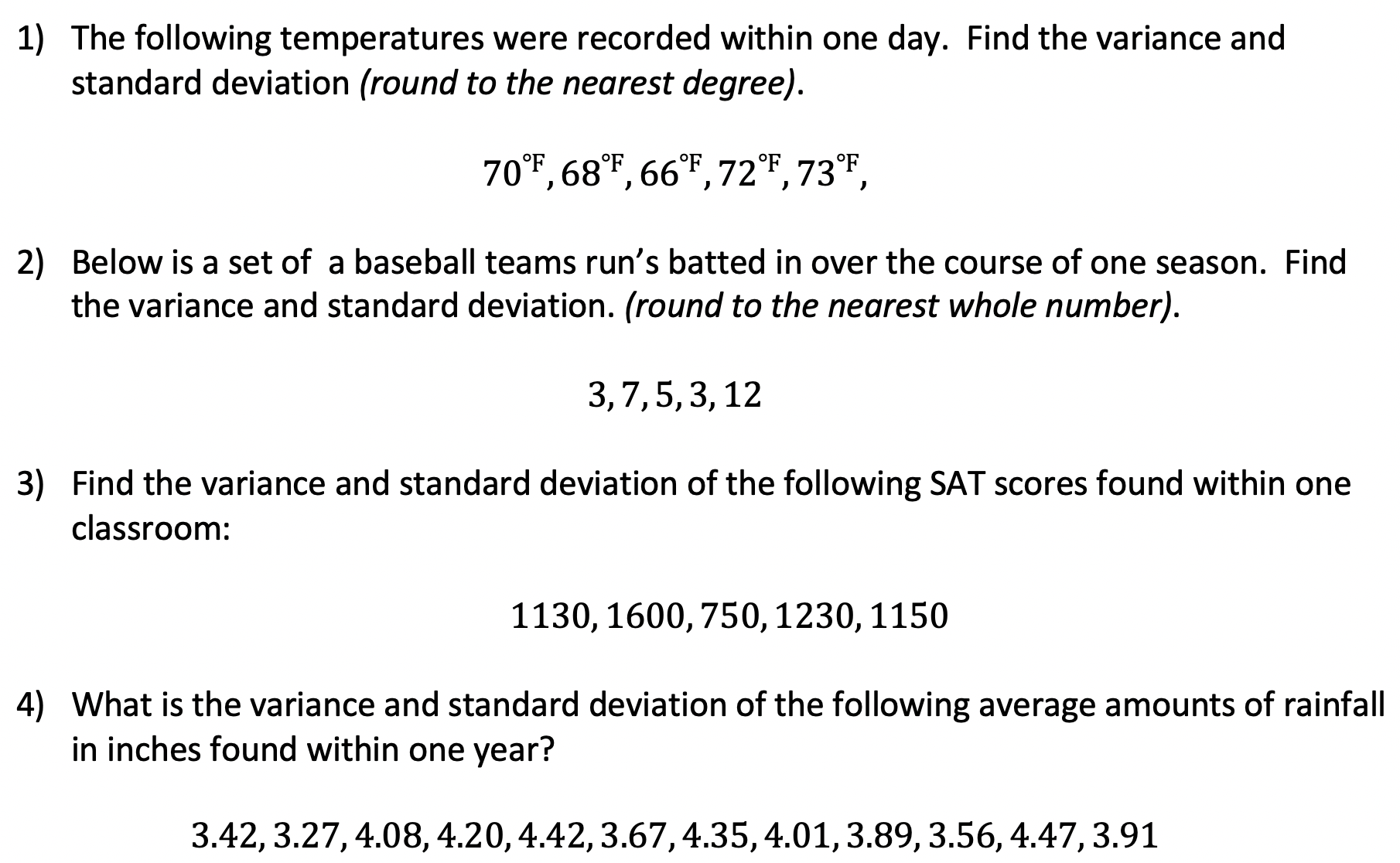
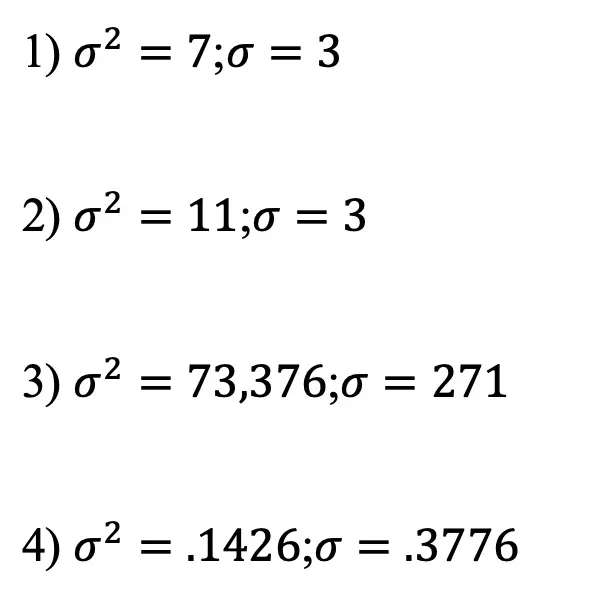
Now try calculating the standard deviation of each data set below on your own with the following practice problems!

Practice Questions:

sample standard deviation

Solutions:

sample standard deviation

Other Related Formulas

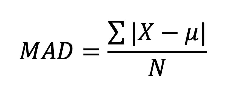
Mean Absolute Deviation (MAD):

The Mean Absolute Deviation otherwise known as MAD is another formula related to variance and standard deviation. In the MAD formula above, notice we are doing very similar steps, by finding the distance to the mean of each data point, only this time we are taking the aboslute value of the ditsance to the mean. Then we sum all the absolute value distances together and divide by the total number of data points.

Why do we use aboslute value in this formula? We take the absolut value, because if didn’t the distance to the means summed togther would cancel eachother out to get zero!

Where…

X = Data point value

μ = mean

N=Total number of data points

|X-μ|=absolute deviation

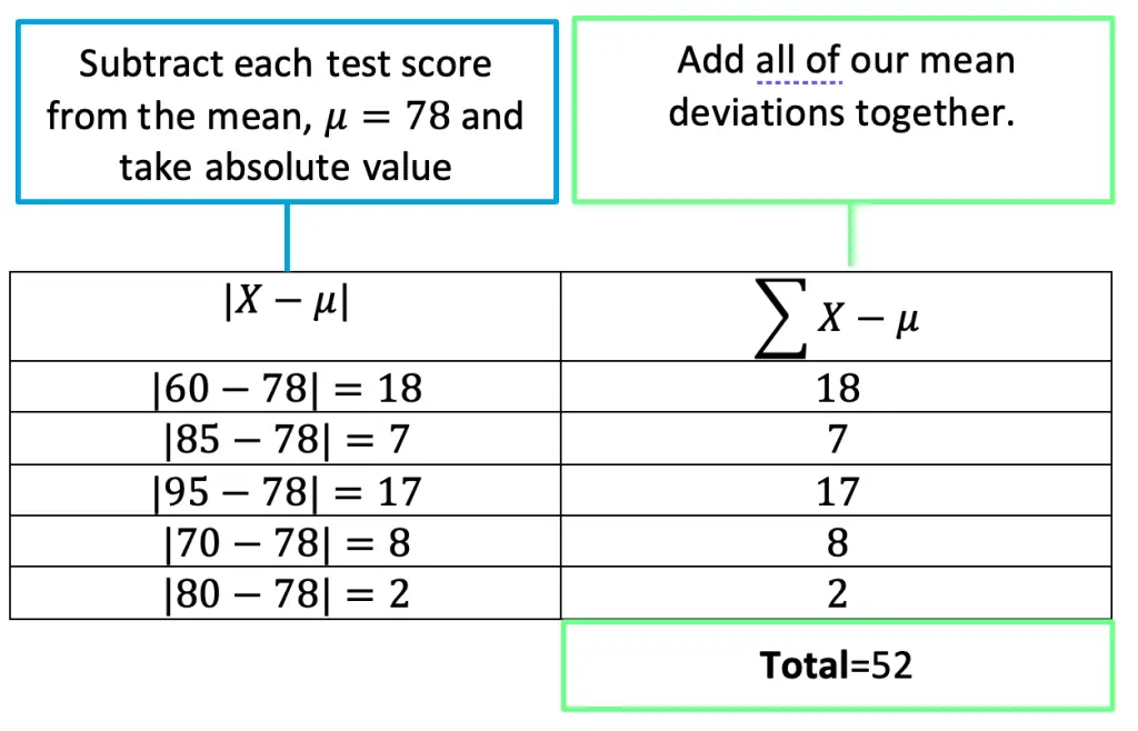
If we were to take the sample from our example earlier,60, 85, 95, 70, 80, in this post and find the MAD it would go something like this:

Expected Value:

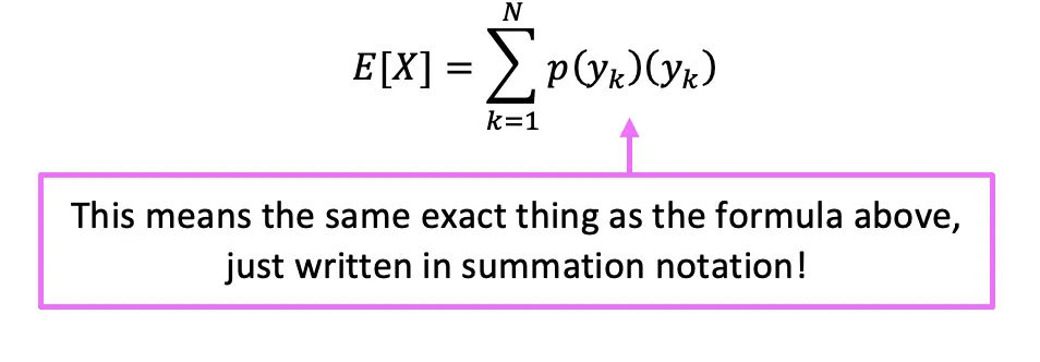
Expected Value is the weighted average of all possible outcomes of one “game” or “gamble” based on the respective probabilities of each potential outcome for a discrete random variable. A “gamble” is defined by the following rules: 1) All possible outcomes are known 2) An outcome cannot be predicted 3) All possible outcomes are of numeric value and 4) The Game can be repeated multiple times under the same conditions.

How to Find Expected Value

Still got questions? No problem! Don’t hesitate to comment with any questions or check out the video above. Happy calculating! 🙂

Facebook ~ Twitter ~ TikTok ~ Youtube

Also! If you’re looking for more statistics, check out this post on how to create and analyze box and whisker plots here!

Combining Like Terms and Distributive Property: Algebra

Greetings math peeps! In today’s post, we are going to review some of the basics: combining like terms and distributive property. It’s so important to master the basics such as these, so you’re prepared and ready to handle the harder stuff that’s just around the corner, trust me they’re coming! And for those who already feel comfortable with these topics, great! Skip ahead and try the practice questions at the bottom of this post and happy calculating! 🙂

When do we combine “like terms?”

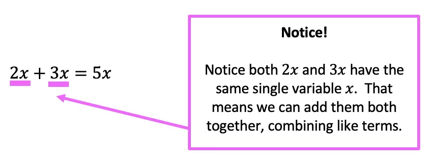
Combining like terms allows us to simplify and calculate our answer with terms that have the same variable and same exponent values only. For example, we can combine the following expression:

distributive property and combining like terms

How do we combine like terms?

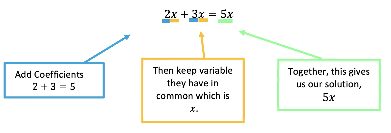
We add or subtract the whole number coefficients and keep the variable they have in common.

distributive property and combining like terms

Why? We could not add these two terms together because their variables do not match! 2 is multiplied by x, while 3 is multiplied by the variable xy.

distributive property and combining like terms

Why? We could not add these two terms together because their variables and exponents do not match! 2 is multiplied by x, while 3 is multiplied by the variable x^2 . Exponents for each variable must match to be considered like terms.

Distributive Property:

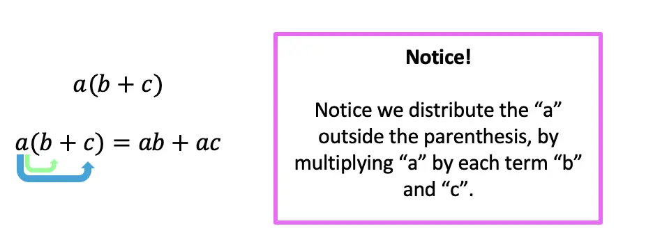
Combining like terms and the distributive property go hand in hand.  The distributive property rule states the following:

distributive property and combining like terms

There are no like terms to combine in the example above, but let’s see what it would like to use the distributive property and combine like terms at the same time with the following examples:

Example #1:

distributive property and combining like terms

Example #2:

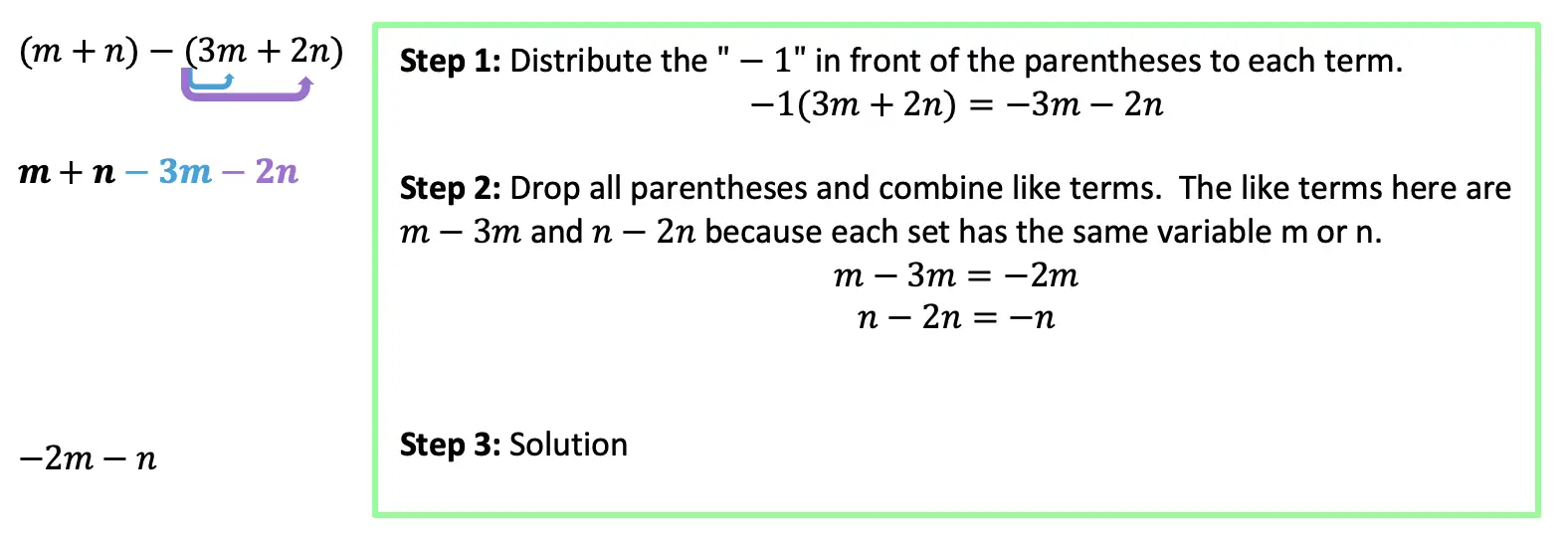
In some cases, we also have to distribute the -1 that can sometimes “hide” behind a parenthesis.

distributive property and combining like terms

Try the following questions on your own on combining like terms and the distributive property and check out the video above for more!

Practice Questions:

Solutions:

Still got questions? No problem! Don’t hesitate to comment with any questions or check out the video above. Happy calculating! 🙂

Looking to review more of the basics? Check out this post on graphing equations of a line y=mx+b here.

Facebook ~ Twitter ~ TikTok ~ Youtube

Box and Whisker Plots, IQR and Outliers: Statistics

Ahoy math friends! This post takes a look at one method of analyzing data; box and whisker plots. Box and whisker plots are great for visually identifying outliers and the overall spread of numbers in a data set. We will go over step by step how to create a box and whisker plot given a set of data, we will then look at how to find the interquartile range and upper and lower outliers. If you have any questions, don’t hesitate to check out the video or comment below. Stay curious and happy calculating! 🙂

Looking for more MathSux? Check out this post on variance and standard deviation here!
Box plots look something like this:

Screen Shot 2020-09-02 at 11.19.22 AM.png

Why Box Plots?

Box Plots are a great way to visually see the distribution of a set of data.  For example, if we wanted to visualize the wide range of temperatures found in a day in NYC, we would get all of our data (temperatures for the day), and once a box plot was made, we could easily identify the highest and lowest temperatures in relation to its median (median: aka middle number).

From looking at a Box Plot we can also quickly find the Interquartile Range and upper and lower Outliers. Don’t worry,  we’ll go over each of these later, but first, let’s construct our Box Plot!
Screen Shot 2020-09-02 at 11.20.42 AM
Screen Shot 2020-09-02 at 11.21.28 AM.png
Box and Whisker Plots

->  First, we want to put all of our temperatures in order from smallest to largest.
-> Now we can find Quartile 1 (Q1), Quartile 2 (Q2) (which is also the median), and Quartile 3 (Q3).  We do this by splitting the data into sections and finding the middle value of each section.

Q1=Median of first half of data

Q2=Median of entire data set

Q3=Median of second half of data

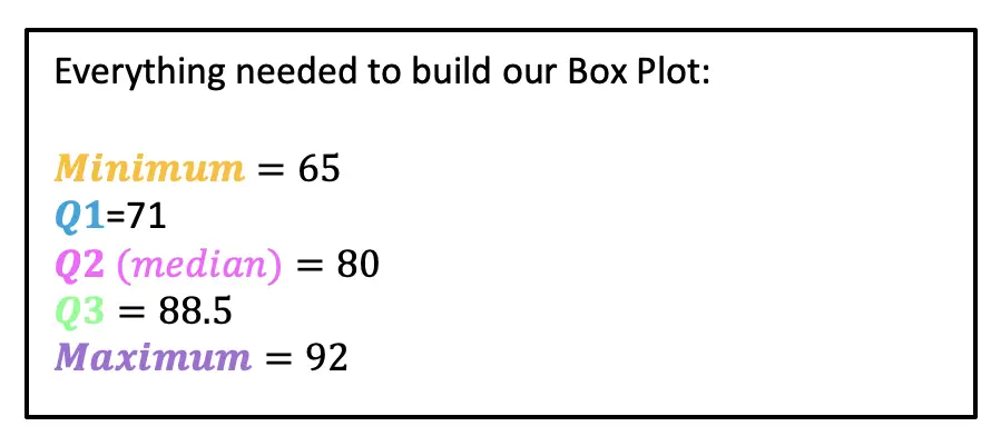
-> Now that we have all of our quartiles, we can make our Box Plot! Something we also have to take notice of, is the minimum and maximum values of our data, which are 65 and 92 respectively. Let’s lay out all of our data below and then build our box plot:

Box and Whisker Plots

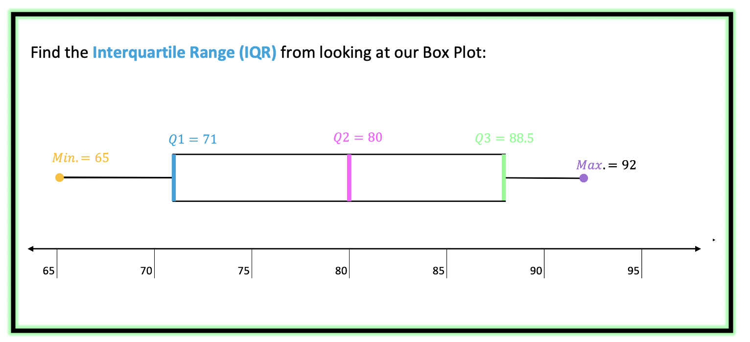
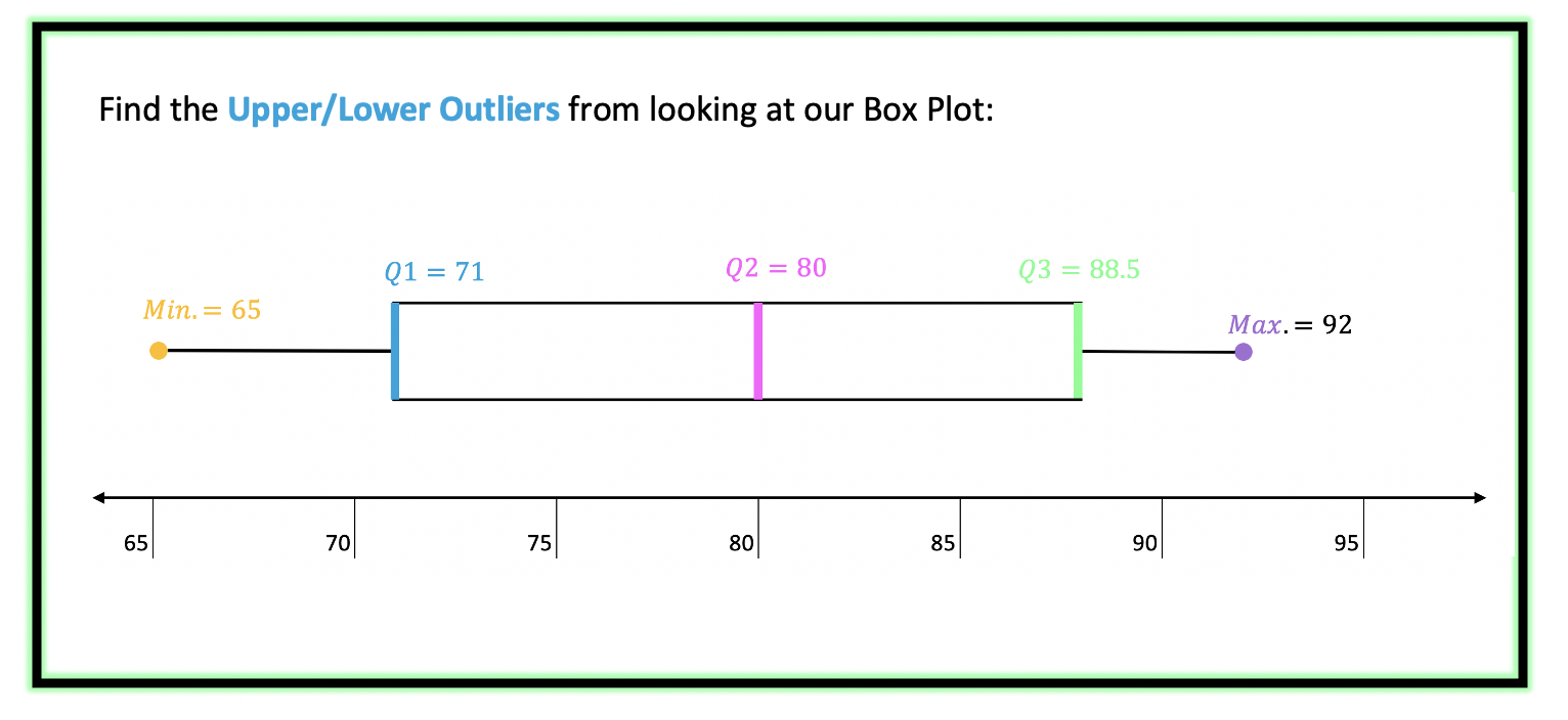
Now that we have our Box Plot, we can easily find the Interquartile Range and upper/lower Outliers.

Screen Shot 2020-09-05 at 11.21.54 PM

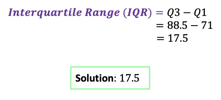
->The Interquartile Range is the difference between Q3 and Q1. Since we know both of these values, this should be easy!

Screen Shot 2020-09-05 at 11.22.02 PM

Next, we calculate the upper/lower Outliers.

Box and Whisker Plots

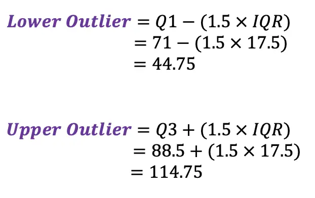
-> The Upper/Lower Outliers are extreme data points that can skew the data affecting the distribution and our impression of the numbers. To see if there are any outliers in our data we use the following formulas for extreme data points below and above the central data points.

Screen Shot 2020-09-05 at 11.24.27 PM

*These numbers tell us if there are any data points below 44.75 or above 114.75, these temperatures would be considered outliers, ultimately skewing our data. For example, if we had a temperature of  Screen Shot 2020-09-05 at 11.26.38 PMor Screen Shot 2020-09-05 at 11.29.25 PM these would both be considered outliers.

Screen Shot 2020-09-05 at 11.24.35 PM

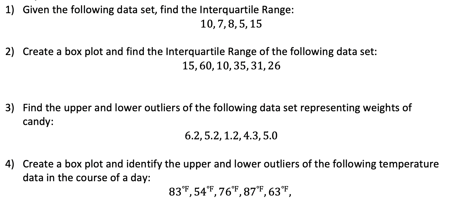
Practice Questions:

Screen Shot 2020-09-05 at 11.34.21 PM

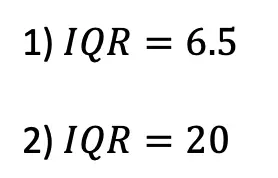
Solutions:

Screen Shot 2020-09-05 at 11.37.06 PM
Box and Whisker Plots
Screen Shot 2020-09-05 at 11.38.10 PM
Box and Whisker Plots

Still got questions? No problem! Don’t hesitate to comment with any questions or check out the video above. Happy calculating! 🙂

Facebook ~ Twitter ~ TikTok ~ Youtube

How to make other Graphs?

Looking to learn about different types of graphs to represent data differently? Check out the difference between Bar Graphs and Histograms here!