Dilations: Scale Factor & Points Other than Origin

Hi there and welcome to MathSux! Today we are going to break down dilations; what they are, how to find the scale factor, and how to dilate about a point other than the origin. Dilations are a type of transformation that are a bit different when compared to other types of transformations out there (translations, rotations, reflections). Once a shape is dilated, the length, area, and perimeter of the shape change, keep on reading to see how! And if you’re looking for more transformations, check out these posts on reflections and rotations. Thanks so much for stopping by and happy calculating! 🙂

What are Dilations?

Dilations are a type of transformation in geometry where we take a point, line, or shape and make it bigger or smaller, depending on the Scale Factor.

We always multiply the value of the scale factor by the original shape’s length or coordinate point(s) to get the dilated image of the shape. A scale factor greater than one makes a shape bigger, and a scale factor less than one makes a shape smaller. Let’s take a look at how different values of scale factors affect the dilation below:

Scale Factor >1 Bigger

Scale Factor <1 Smaller
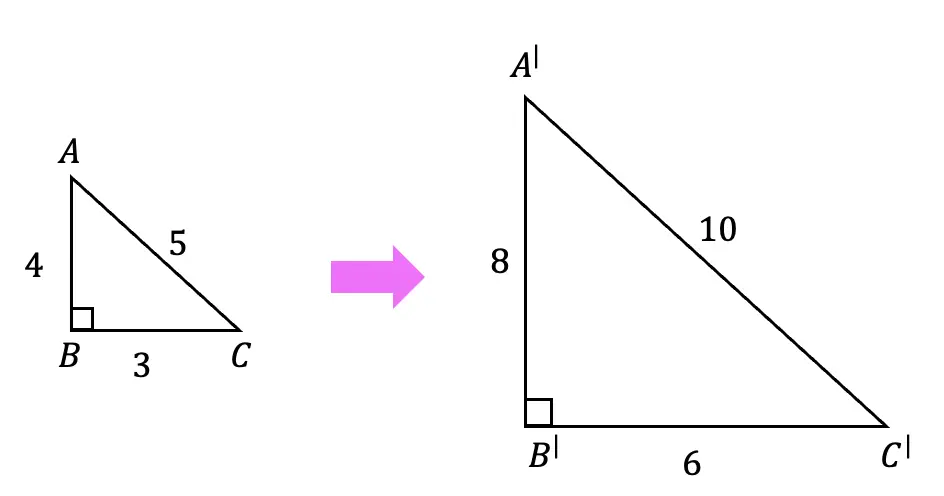
Scale Factor=2

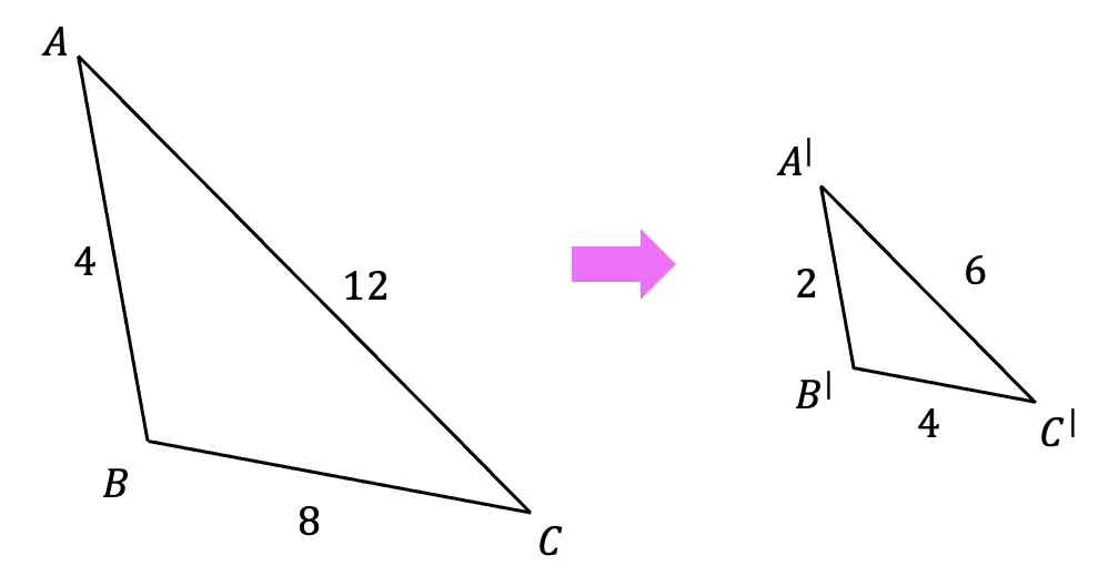
 In the below diagram the original triangle ABC gets dilated by a scale factor of 2.  Notice that the triangle gets bigger, and that each length of the original triangle is multiplied by 2.

Dilations

Scale Factor=1/2

Here, the original triangle ABC gets dilated by a scale factor of 1/2.  Notice that the triangle gets smaller, and that each length of the original triangle is multiplied by 1/2 (or divided by 2).

Dilations

Properties of Dilations:

There are few things that happen when a shape and/or line undergoes a dilation.  Let’s take a look at each property of a dilation below:

1. Angle values remain the same.

2. Parallel and perpendicular lines remain the same.

3. Length, area, and perimeter do not remain the same.

Now that we a bit more familiar with how dilations work, let’s look at some examples on the coordinate plane:

Example #1: Finding the Scale Factor

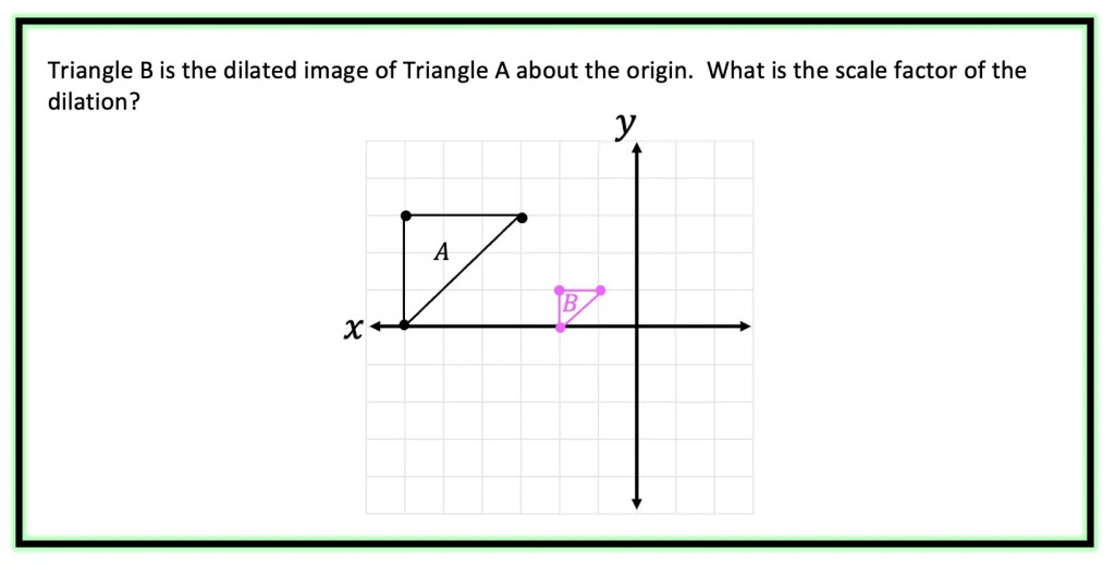
Step 1: First, let’s look at two corresponding sides of our triangle and measure their length.

Dilations

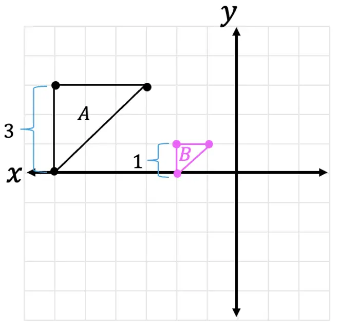
Step 2: Now, let’s look at the difference between the two lengths and ask ourselves, how did we go from 3 units to 1 unit?

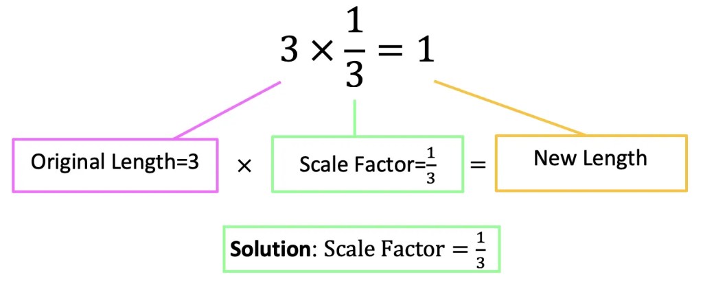
Remember, we are always multiplying the scale factor by the original length values in order to dilate an image. Therefore, we know we must have multiplied the original length by 1/3 to get the new length of 1.

Dilations

When it comes to dilations, there are different types of questions we may be faced with.  In the last question, the triangle dilated was done so about the origin, but this won’t always be the case.  Let’s see how to dilate a point about a point other than the origin with this next example.

Example #2: Dilating about a Point other than the Origin

Dilations

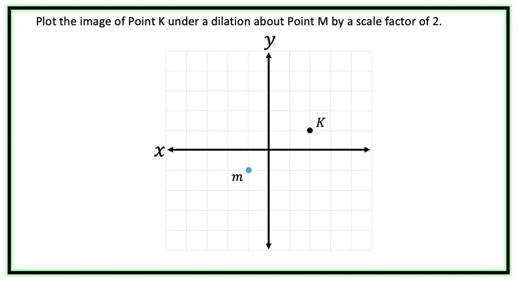
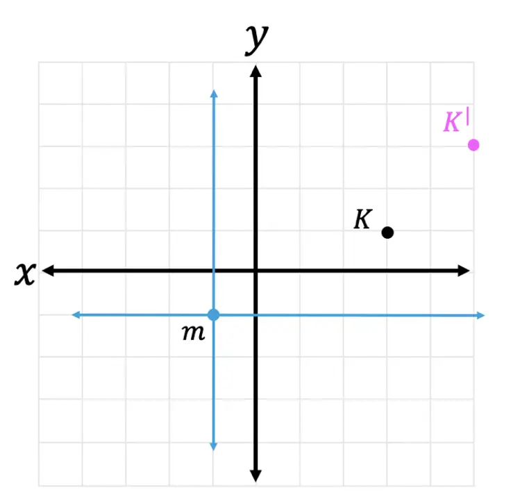
Step 1: First, let’s look at our point of dilation, notice it is not at the origin! In this question, we are dilating about point m!  To understand where our triangle is in relation to point m, let’s draw a new x and y axes originating from this point in blue below.

Dilations

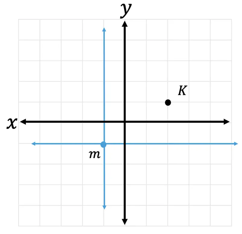
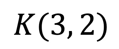
Step 2: Now, let’s look at coordinate point K, in relation to our new axes.

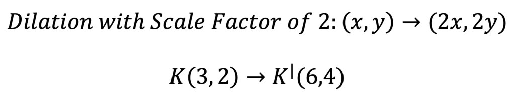
Step 3: Let’s use the scale factor of 2 and the transformation rule for dilation, to find the value of its new coordinate point. Remember, in order to perform a dilation, we multiply each coordinate point by the scale factor.

Step 4: Finally, let’s graph the dilated image of coordinate point K. Remember we are graphing the point (6,4) in relation to the x and y-axis that stems from point m.

Dilations

Check out these dilation questions below!

Practice Questions:

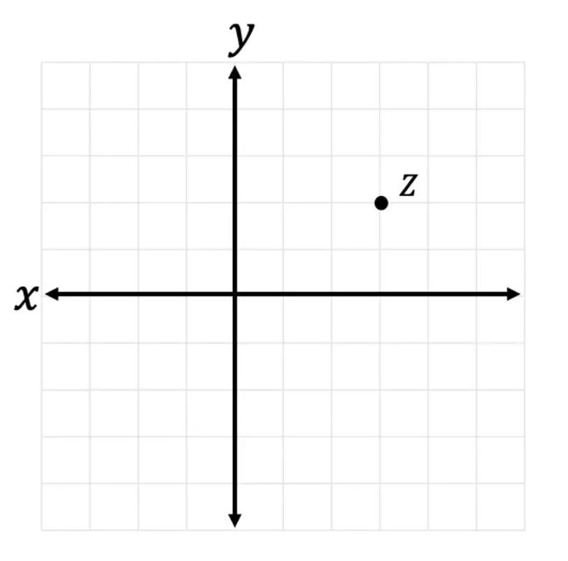
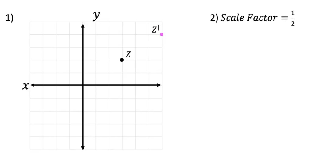
1) Plot the image of Point Z under a dilation about the origin by a scale factor of 2.

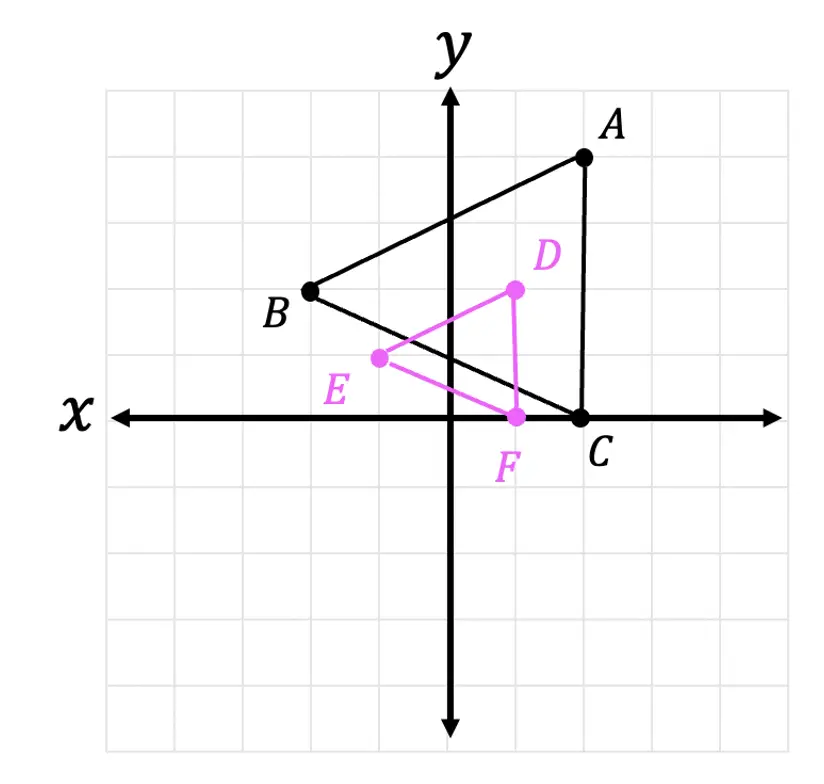
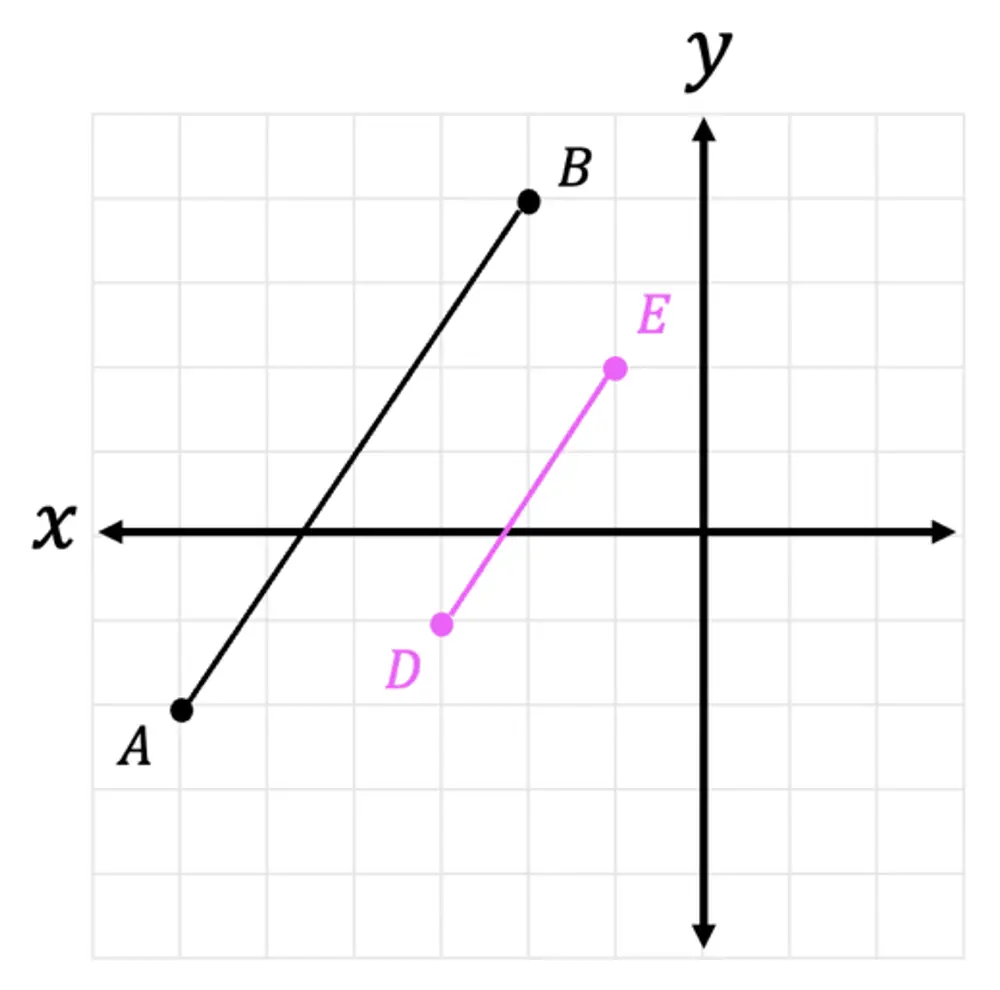
2) Triangle DEF is the image of triangle ABC after a dilation about the origin. What is the scale factor of the dilation?

Dilations

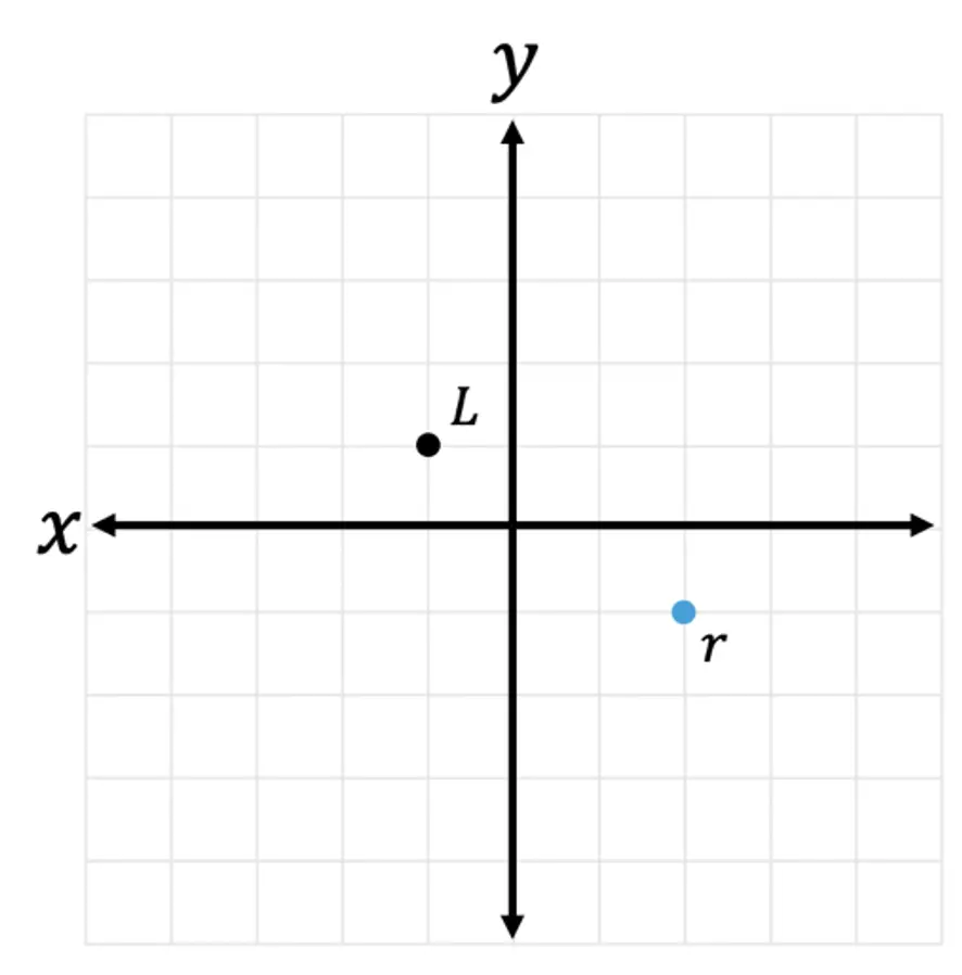
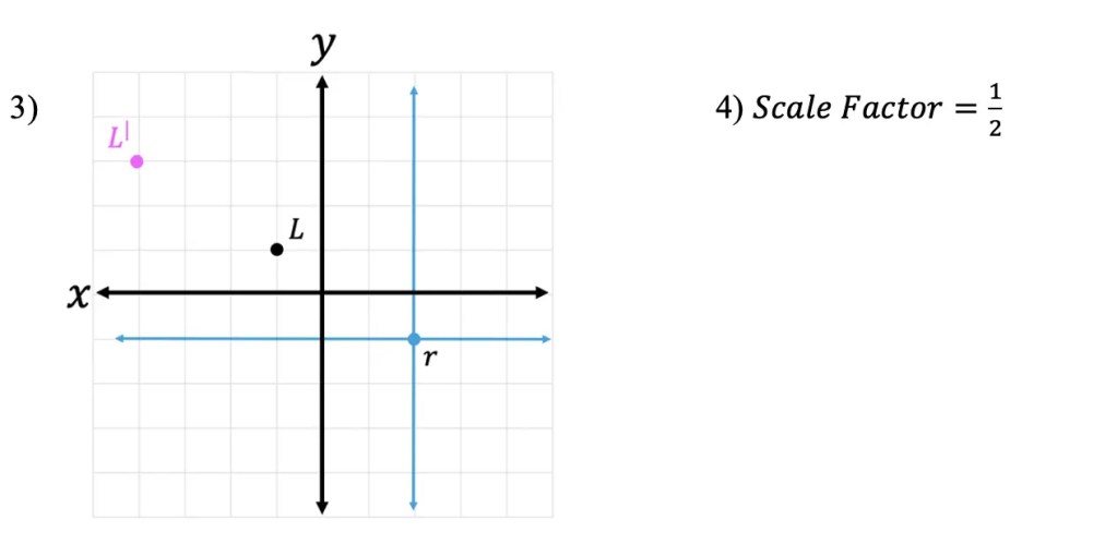
3) Point L is dilated by a scale factor of 2 about point r. Draw the dilated image of point L.

Dilations

4) Line DE is the dilated image of line AB. What is the scale factor of the dilation?

Solutions:

Still got questions? No problem! Don’t hesitate to comment with any questions below. Thanks for stopping by and happy calculating! 🙂

Facebook ~ Twitter ~ TikTok ~ Youtube

Looking for more Transformations? Check out the related posts below!

Translations

Rotations

Reflections

What is the Discriminant?

Hi everyone and welcome to MathSux! In this post, we are going to answer the question, what is the discriminant? Before going any further, if you need a review on what the quadratic equation or imaginary numbers are, check out each related link! Also, don’t forget to check out the video and practice questions below. Happy calculating! 🙂

What is the Discriminant?

The discriminant is a formula we can use that tells us more about a quadratic equation including:

  1. The number of solutions a quadratic equation has.
  2. The “nature” of the roots of the solution (rational/irrational or real/imaginary).

Discriminant Formula:

The discriminant formula may look familiar! It is part of the quadratic formula and we have seen it before, using the very same coefficients a, b, and c from the quadratic equation.

What is the Discriminant?

How does it Work?

When we find the value of the discriminant of any quadratic equation, it will give us a value that tells us how many solutions (or roots) a quadratic equation has.  Remember when we say “roots” what we really mean are the x-value(s) of the quadratic equation that hit the x-axis. This value will also tell us if the solutions to the quadratic equation are rational/irrational or real/imaginary. Take a look at how it all breaks down below:

Now that we are familiar with the rules, let’s take a look at an Example:

Step 1: First let’s write out our quadratic equation and identify the coefficients a, b, and c so they are ready to be plugged into our discriminant formula.

Step 2: Now let’s write out and fill in our formula using the coefficients and solve.

What is the Discriminant?

Step 3: Now let’s analyze our answer! Since, we got a discriminant value of 36, notice that it is a positive perfect square! If we look back at our discriminant table, this tells us that our quadratic equation is going to have 2 real and rational solutions.

Practice Questions:

Find the discriminant, number of solutions and nature of the roots of the following quadratic equations:  

Solutions:

Still got questions? No problem! Don’t hesitate to comment with any questions below or check out the video above. Thanks for stopping by and happy calculating! 🙂

Facebook ~ Twitter ~ TikTok ~ Youtube

Looking for more on Quadratic Equations and Functions? Check out the following Related posts!

Factoring Review

Factor by Grouping

Completing the Square

4 Ways to Factor a Trinomial

Is it a Function?

Imaginary and Complex Numbers

Focus and Directrix of a Parabola

Quadratic Equations with 2 Imaginary Solutions

Factor By Grouping Examples: Algebra

Hey there math peeps and welcome to MathSux! In today’s post we are going to cover factor by grouping examples, a surprisingly cool and easy factoring method used to factor quadratic equations when “a” is greater than one. It can also be used to factor four term polynomials. We are going to look at an example of each below. If you have any questions, please don’t hesitate to check out the video and try the practice problems at the end of this post. Thanks for stopping by and happy calculating! 🙂

What is Factor by Grouping?

Factor by Grouping is a factoring method that groups common factors of an algebraic expression together.  Many times, we use factoring to find the x-values of a quadratic equation when the coefficient “a” is greater than 1.

When should we use Factor by Grouping?

1) If the first coefficient in a quadratic equation, a, is greater than 1:

Factor By Grouping examples

2) When there is a polynomial with 4 terms:

Factor by Grouping Examples:

Ready for an Example?  Let us look at how to factor a quadratic equation when a is greater than one.

Factor By Grouping examples

Now, let’s take a look at another type of example, that can be solved with the help of factor by grouping!

Notice that this question is actually easier to solve than the last! The polynomial above, is already split into 4 terms, therefore, we can jump ahead, skipping the product/sum steps we did in the previous example!

Factor By Grouping examples

Ready to try practice questions on your own? Check them out below to master Factor by Grouping!

Practice Questions:

Solutions:

Still got questions? No problem! Don’t hesitate to comment with any questions below. Thanks for stopping by and happy calculating! 🙂

Facebook ~ Twitter ~ TikTok ~ Youtube

Looking to learn about different Factoring methods and functions? Check out the related posts below!

GCF, Product/Sum, Difference of Two Squares, Quadratic Formula

Quadratic Formula, Product/Sum, Completing the Square, Graph

Completing the Square

The Discriminant

Is it a Function?

Quadratic Equations with 2 Imaginary Solutions

Free High School Math Resources

Free High School Math Resources

Greetings math friends! Today’s post is for the New York state teachers out there in need of a lesson boost. In this post, we’ll go over what MathSux has to offer for free high school math resources including videos, lessons, practice questions, etc. Remember everything you see here is 100% free and designed to make your life (and your students’ life) easier.

Signing up with MathSux will get you access to FREE:

1) Math Videos

2) Math Lessons

3) Practice Questions

4) NYS Regents Review

Everything designed here aligns with the NYS Common Core Standards for Algebra, Geometry, Algebra 2/Trig. and Statistics.

I am a NYS math teacher that creates free math videos, lessons, and practice questions every week, right here, for you! On the YouTube channel, you’ll also find NYS Common Core Regents questions reviewed one question at a time.

Featured on Google Classrooms around the world, MathSux.org is a great resource especially now, in the time of COVID and zooming and schooling from home. I hope you stick around and find these resources helpful.

And if you’re looking to get the latest MathSux.org videos and emails straight to your inbox, don’t forget to sign up on the right hand-side of the website. Thanks so much for stopping by and happy calculating! 🙂

Facebook ~ Twitter ~ TikTok ~ Youtube

Bisect a Line Segment

Hi everyone and welcome to MathSux! In this post we are going to be constructing a perpendicular bisector by using a compass and stright edge. A perpendicular bisector, (also known as a segment bisector), is a line that cuts a line segment in half and creates four 90º angles. It is a super fast and super simple construction! We’ll also go over the Perpendicular Bisector Theorem we can infer from our original construction. If you’re looking for more geometric constructions, don’t forget to check more out here. Thanks so much for stopping by and happy calculating! 🙂

What is the Perpendicular Bisector of a line segment?

  • A perpendicular bisector slices our line segment AB (or any line segment) in half at its midpoint, creating two equal halves.
  • This will also create a 90º angle ( or right angle) about the line.
Constructing a Perpendicular Bisector through line segment AB

What is happening in this GIF?

Step 1: Notice we are given line segment AB. First, we are going to measure out a little more than halfway across the line segment AB by using a compass.

Step 2: Next we are going to place the point of the compass on point A and swing above and below line segment AB to create a half circle.

Step 3: Keeping the same distance on our compass, we are then going to place the point of the compass onto Point B (the opposite side) and repeat the same step we did on point A, drawing an arc in the shape of a semi-circle.

Step 4: Notice the intersection point above and below line segment AB!? Now, we are going to connect these two points by drawing a line with a ruler or straightedge.

Step 5: Yay! We now have a segment bisector! This cuts line segment AB right at its midpoint, while also dividing line segment AB into two equal halves and creating a 90º angle around our two intersecting lines.

Perpendicular Bisector Theorem:

The Perpendicular Bisector Theorem explains that any point along the perpendicular bisector line we just create is equidistant to each end point of the original line segment (in this case line segment AB).

Therefore, if we were to draw points C,D, and E along the perpendicular bisector, then draw imaginary lines stemming from these points to each end point, we’d get something like the image below:

AC = CB

AD = DB

AE = EB

Line Segment Theorem

Notice that with each of our points on the perpendicular line above, we can now state that the following is true:

AC = CB

AD = DB

AE = EB

The fact that we can state the above is true is reason for the Perpendicular Bisector Theorem!

Constructions and Related Posts:

Looking to construct more than just a perpendicular segment bisector? Check out these related posts and step by step tutorials on geometry constructions below!

Construct an Equilateral Triangle

Perpendicular Line through a Point

Angle Bisector

Construct a 45º angle

Altitudes of a Triangle (Acute, Obtuse, Right)

Construct a Square inscribed in a Circle

Best Geometry Tools!

Looking to get the best construction tools? Any compass and straight edge will do the trick, but personally, I prefer to use my favorite mini math toolbox from Staedler. Stadler has a geometry math set that comes with a mini ruler, compass, protractor, and eraser in a nice travel-sized pack that is perfect for students on the go and for keeping everything organized….did I mention it’s only $7.99 on Amazon?! This is the same set I use for every construction video! Check out the link below and let me know what you think!

Still got questions? No problem! Don’t hesitate to comment with any questions below or check out the video above. Thanks for stopping by and happy calculating! 🙂

Facebook ~ Twitter ~ TikTok ~ Youtube

Want to see how to construct a square inscribed in a circle? Or maybe you want to construct an equilateral triangle? Click on each link to view each construction! And if you’re looking for even more geometry constructions, check out the link here! And if you’re looking for a construction you don’t yet see, please be sure to suggest it in the comments below!

Square Inscribed in a Circle Construction

Greetings math friends and welcome to MathSux! In this week’s post, we are going to take a step-by-step look at how a square inscribed in a circle construction works! Within this post we have a video, a GIF, and a step-by-step written explanation below, the choice of learning how to do this construction is up to you! Happy Calculating! 🙂

Square Inscribed in a Circle Construction

How to Construct a Square Inscribed in Circle:

Step 1: First, we are going to draw a circle using a compass (any size).

Step 2: Using a ruler, draw a diameter or straight line across the length of the circle, going through its midpoint.

Step 3: Next, open up the compass across the circle. Then take the point of the compass to one end of the diameter and swing the compass above the circle, creating an arc.

Step 4: Keeping that same length of the compass, go to the other side of the diameter and swing above the circle again making another arc until the two arcs intersect.

Step 5: Now, we are going to repeat steps 3 and 4, this time creating arcs below the circle using the same compass size.

Step 6: Connect the point of intersection above and below the circle using a ruler or straight edge. This creates a perpendicular bisector, cutting the diameter in half and forming a 90º angle.

Step 7: Lastly, we are going to use a ruler to connect each corner point to one another creating a square!

Constructions and Related Posts:

Looking to construct more than just a square inside a circle? Check out these related posts and step-by-step tutorials on geometry constructions below!

Construct an Equilateral Triangle

Perpendicular Line Segment through a Point

Angle Bisector

Construct a 45º angle

Altitudes of a Triangle (Acute, Obtuse, Right)

How to Construct a Parallel Line

Bisect a Line Segment

Best Geometry Tools!

Looking to get the best construction tools? Any compass and straight-edge will do the trick, but personally, I prefer to use my favorite mini math toolbox from Staedler. Stadler has a geometry math set that comes with a mini ruler, compass, protractor, and eraser in a nice travel-sized pack that is perfect for students on the go and for keeping everything organized….did I mention it’s only $7.99 on Amazon?! This is the same set I use for every construction video in this post. Check out the link below and let me know what you think!

Still got questions? No problem! Don’t hesitate to comment with any questions or concerns below. Also if you’re looking for a different type of construction you don’t yet see here, please let me know! Happy calculating! 🙂

Let’s be friends! Check us out on the following social media platforms for even more free MathSux practice questions and videos:

Facebook ~ Twitter ~ TikTok ~ Youtube

Looking for something similar to square inscribed in a circle construction? Check out this post here on how to construct and equilateral triangle here! And if you’re looking for even more geometry constructions, check out the link here!

Simultaneous Equations: Algebra

Happy new year and welcome to Math Sux! In this post we are going to dive right into simultaneous equations and how to solve them three different ways! We will go over how to solve simultaneous equations using the (1) Substitution Method (2) Elimination Method and (3) Graphing Method. Each and every method leading us to the same exact answer! At the end of this post don’t forget to try the practice questions choosing the method that best works for you! Happy calculating! 🙂

What are Simultaneous Equations?

Simultaneous Equations are when two equations are graphed on a coordinate plane and they intersect at, at least one point.  The coordinate point of intersection for both equation is the answer we are trying to find when solving for simultaneous equations. There are three different methods for finding this answer:

We’re going to go over each method for solving simultaneous equations step by step with the example below:

Method #1: Substitution

The idea behind Substitution, is to solve for 1 variable first algebraically, and the plug this value back into the other equation solving for one variable.  Then solving for the remaining variable.  If this sounds confusing, don’t worry! We’re going to do this step by step:

Step 1: Let’s choose the first equation and move our terms around to solve for y.

Simultaneous Equations

Step 3: The equation is set up and ready to solve for x!

Simultaneous Equations

Step 4: All we need to do now, is plug x=3 into one of our original equations to solve for y.

Simultaneous Equations

Step 5: Now that we have solved for both x and y, we have officially found where these two simultaneous equations meet!

Simultaneous Equations

Method #2: Elimination

The main idea of Elimination is to add our two equations together to cancel out one of the variables, allowing us to solve for the remaining variable.  We do this by lining up both equations one on top of the other and adding them together.  If variables at first do not easily cancel out, we then multiply one of the equations by a number so it can. Check out how it’s done step by step below!

Step 1: First, let’s stack both equations one on top of the other to see if we can cancel anything out:

Simultaneous Equations

Step 2: Our goal is to get a 2 in front of y in the first equation, so we are going to multiply the entire first equation by 2.

Simultaneous Equations

Step 3: Now that we multiplied the entire first equation by 2, we can line up our two equations again, adding them together, this time canceling out the variable y to solve for x.

Simultaneous Equations

Step 4: Now, that we’ve found the value of variable x=3, we can plug this into one of our equations and solve for missing unknown variable y.

Simultaneous Equations

Step 5: Now that we have solved for both x and y, we have officially found where these two simultaneous equations meet!

This image has an empty alt attribute; its file name is Screen-Shot-2020-12-30-at-10.21.46-AM.png

Method #3: Graphing

The main idea of Graphing is to graph each a equation on a coordinate plane and then see at what point they intersect.  This is the best method to visualize and check our answer!

Step 1: Before we start graphing let’s convert each equation into y=mx+b (equation of a line) form.

Equation 1:

Equation 2:

Step 2: Now, let’s graph each line, y=3x-4 and y=-x+8, to see at what coordinate point they intersect.

Simultaneous Equations

Need to review how to draw an equation of a line? Check out this post here! Notice we got the same exact answer using all three methods (1) Substitution (2) Elimination and (3) Graphing.

Ready to try the practice problems on your own?! Check them out below!

Practice Questions:

Solve the following simultaneous equations for x and y.

Solutions:

  1. (1, 3)
  2. (4,5)
  3. (-1, -6)
  4. (3, -3)

Want more MathSux?  Don’t forget to check out our Youtube channel and more below! And if you have any questions, please don’t hesitate to comment below. Happy Calculating!

Facebook ~ Twitter ~ TikTok ~ Youtube

If you are looking for a challenge, try solving three equations with three unknown variables, in this post here!

30 60 90 Triangle

Hi everyone and welcome to MathSux! In this post, we are going to break down 30 60 90 degree special right triangles. What is it? Where did it come from? What are the ratios of its side lengths and how do we use them? You will find all of the answers to these questions about this right angled triangle in this post. Also, don’t forget to check out the video below and practice questions at the end of this post to truly become a 30 60 90 special right triangle master! Happy calculating! 🙂

If you want to learn about the other special triangle, 45 45 90 triangle, check out this post here. And if you’re looking to make math suck just a little bit less? Subscribe to our Youtube channel for free math videos every week! 🙂

Facebook ~ Twitter ~ TikTok ~ Youtube

30 60 90 Triangle Ratio:

30 60 90 triangle side lengths

Notice that the 30 60 90 triangle is made up of one right angle across from the hypotenuse (which is always going to be the longest side), a 60 degree angle with a longer leg on the opposite side, and a 30 degree angle measure across from the shorter leg.

What is a 30 60 90 Triangle and why is it “Special”?

The 30 60 90 triangle is a special right triangle because it forms an equilateral triangle when a mirror image of itself is drawn. This means that all sides are equal when a mirror image of the triangle is drawn which allows us to find the ratio between each of the sides of the triangle by using the Pythagorean Theorem. Check it out below!

30 60 90 Special Triangles

Now let’s draw a mirror image of our triangle to create an equilateral triangle.  Next, we can label the length of the new side opposite 30 degrees (the shorter leg) “a,” and add this new mirror image length with the original we had to get, a total of a+a=2a.

30 60 90 Special Triangles

If we look at our original 30 60 90 triangle, we now have the following values for each side based on our equilateral triangle. Notice we still need to find the length value of the longer leg, opposite angle 60 degrees.

30 60 90 Special Triangles
Pythagorean Theorem Formula
Fill in values from our triangle longer leg
Distribute the exponent and start solving for our “?” by subtracting a^2 from both sides.
Now take the square root of both sides to solve for “?.”	We have found a solution! Our missing side length is equal to a√3.

To sum up, we have applied the Pythagorean Theorem formula, filled in values found in our triangle for each length, distributed the exponent and subtracted a2 from both sides, took the square root, and finally found our solution for our ratio for the longer leg opposite 60 degrees.

Now we can re-label our triangle, knowing the length of the hypotenuse in relation to the two legs. This creates a ratio that applies to all 30 60 90 triangles!

30 60 90 triangle side lengths

How do I use this ratio?

30 60 90 triangle side lengths

Knowing the above ratio, allows us to find any length of any and every 30 60 90 triangle, when given the value of one of its sides. Let’s tsee how this ratio works with some examples.

Example #1:

30 60 90 triangle side lengths

Step 1: First let’s look at our ratio and compare it to our given triangle.

30 60 90 triangle side lengths

Step 2: Notice we are given the value of a, which is equal to 4, knowing this we can now fill in each length of our triangle based on the ratio of a 30 60 90 triangle.

30 60 90 triangle side lengths

Now let’s look at another Example where we are given the length of the hypotenuse and need to find the values of the other two missing sides.

Example #2:

30 60 90 triangle side lengths

Step 1: First let’s look at our ratio and compare it to our given triangle.

30 60 90 triangle side lengths

Step 2: Notice we are given the value of the hypotenuse, 2a=20. Knowing this we can find the value of a by dividing 20 by 2 to get a=10. Once we have the value of a=10, we can easily find the length of the last, longer leg based on the 30 60 90 ratio:

30 60 90 triangle side lengths

Now for our last Example, we will see how to find the value of the shorter leg and hypotenuse, when we are given the side length of the longer leg across from 60º and need to find the other two missing sides.

Example #3:

30 60 90 triangle side lengths

Step 1: First let’s look at our ratio and compare it to our given triangle.

30 60 90 triangle side lengths

Step 2: In this case, we need to use little algebra to find the value of a, using the ratio for 30 60 90 triangles.

30 60 90 triangle side lengths
We set up this equation, knowing that 9 is across from 60 degrees, and that a√3=9. 	To solve for a, we divide square root both sides by √3. 	We get a solution a=9/√3! Yay! We cannot have a radical in the denominator, so we rationalize the denominator by multiplying the numerator and denominator by √3.

Now that we have one piece of the puzzle, the value of a, let’s fill in the value of the shorter leg of our triangle below:

Finally, let’s find the value of the length of the hypotenuse, which is equal to 2a in our ratio. Knowing the length of all sides, we can fill in the lengths of each side of our triangle for our solution.

Think you are ready to master these types of questions on your own? Try the practice problems below!

Practice Questions:

Find the value of the missing sides of each 30 60 90 degree triangle.

Solutions:

Still got questions? No problem! Don’t hesitate to comment with any questions or check out the video above. Happy calculating! 🙂

Facebook ~ Twitter ~ TikTok ~ Youtube

Related Trigonometry Posts:

The Unit Circle

Basic Right Triangle Trigonometric Ratios (SOH CAH TOA)

4545 90 Special Triangles

Factoring Trigonometric Functions

Graphing Trigonometric Functions

Trig Identities

Transforming Trig Functions

Law of Cosines

Law of Sines

Transforming Trig Functions: Amplitude, Frequency, Period, Phase Shifts

Hi everyone, and welcome to MathSux! In this post, we are going to break down transforming trig functions by identifying their amplitude, frequency, period, horizontal phase shift, and vertical phase shifts. Fear not! Because we will break down what each of these terms (amplitude, frequency, period, horizontal phase shift and vertical phase shifts) mean and how to find them when looking at a trigonometric function and then apply each of these changes step by step to our graph. In this particular post, we will be transforming and focusing on a cosine function, but keep in mind that the same rules apply for transforming sine functions as well (example shown below in practice).

And if you’re ready for more, check out the video and the practice problems below, happy calculating! 🙂

*For a review on how to derive the basic Trig functions (y=sinx, y=cosx, and y=tanx), click here.

What are the Different Parts of a Trig Function?

When transforming trig functions, there are several things to look out for, let’s take a look at what each part of a trig function represents below:

Trig functions

Amplitude: The distance (or absolute value) between the x axis and the highest point on the graph.

Frequency: This is the number of cycles that happen between 0 and 2π. (Α “cycle” in this case is the number of “s” cycles for the sine function).

Period: The x-value/length of one cycle. (Α “cycle” in this case is the number of “s” cycles for the sine function). This is found by looking at the graph and seeing where the first cycle ends, or, by using the formula:       

Horizontal Shift: When a trigonometric function is moved either left or right along the x axis.

Vertical Shift: When a trigonometric function is moved either up or down along the y axis.

Let’s try an Example, by graphing the following trig function step by step by identifying the amplitude, frequency, period, vertical shift, and horizontal phase shift.

Step 1: First let’s label and identify all the different parts of our trig function and what each part represents.

Trig functions

Step 2: Now let’s transform our trig graph one step at a time.  First, let’s start graphing y=cos(x) without any transformations, the basic graph.

Trig functions
Graph y=cos(x)

Step 3: Next, let’s add our amplitude of 2, otherwise known as the height, or distance to the x-axis.  To do this our highest and lowest points on the y-axis will now be moved to 2 and -2 respectively. 

Trig functions
Re-draw y=cos(x), with an amplitude of 2 to get y=2cos(x)

Step 4: Next, we can apply our horizontal shift to the left by (π/2) or 90º.  To do this, we need to look at where negative (π/2) is on our graph at (-π/2) and move our entire graph over to start at this new point, “shifting” over each coordinate point by (π/2) along the x axis.

Trig functions
Shift our graph y=2cos(x) over by 90º to the left to get y=2cos(x+(π/2))

Step 5: For our last transformation, we have a vertical phase shift up 1 unit.  All this means is that we are going to shift our entire graph up by 1 unit along the y axis.

Trig function graph
phase shift
vertical shift
Shift our entire graph y=2cos(x+(π/2)) up one unit along the y-axis to get y=2cos(x+(π/2))+1

Think you are ready to try graphing trig functions and identifying the amplitude, frequency, period, vertical phase shift, and horizontal phase shift? Check out the practice questions and answers below!

Practice Questions:

When you’re ready check out the function transformations solutions below:

Solutions:

Still, got questions? No problem! Don’t hesitate to comment with any questions or check out the video above for an in-depth explanation. Happy calculating! 🙂

Facebook ~ Twitter ~ TikTok ~ Youtube

Related Trigonometry Posts:

The Unit Circle

Basic Right Triangle Trigonometric Ratios (SOH CAH TOA)

4545 90 Special Triangles

30 60 90 Special Triangles

Graphing Trigonometric Functions

Trig Identities

Factoring Trigonometric Functions

Law of Cosines

Law of Sines

Graphing Linear Inequalities: Algebra

graphing linear inequalities

Hi and welcome to MathSux! In this post, we are going to go over the rules for graphing linear inequalities on a coordinate plane when it comes to drawing lines, circles , and shading, then we are going to solve an example step by step. If you have any questions, check out the video below and try the practice questions at the end of this post! If you still have questions, don’t hesitate to comment below and happy calculating! 🙂

Graphing Linear Inequalities:

When graphing linear inequalities, we always want to treat the inequality as an equation of a line in  form y=mx+b….with a few exceptions:

Graphing Linear Inequalities
inequality shading above or below y-axis

Now that we know the rules, of graphing inequalities, let’s take a look at an Example!

Graphing Linear Inequalities Example:

graphing inequality example

Step 1: First, let’s identify what type of inequality we have here.  Since we are working with a > sign, we will need to use a dotted line and open circles when creating our graph.

graphing inequality example

Step 2: Now we are going to start graphing our linear inequality as a normal equation of a line, by identifying the slope and the y-intercept only this time keeping open circles in mind.  (For a review on how to graph regular equation of a line in y=mx+b form, click here)

graphing inequality example
graphing linear inequalities

Step 3: Now let’s connect our dots, by using a dotted line to represent our greater than sign.

graphing linear inequalities

Step 4: Now it is time for us to shade our graph, since this is an inequality, we need to show all of our potential solutions with shading.  Since we have a greater than sign, , we will be shading above the y-axis.  Notice all the positive y-values above are included to the left of our line.  This is where we will shade.

graphing linear inequalities

Step 5: Check!  Now we need to check our work.  To do that, we can choose any point within our shaded region, if the coordinate point we chose hold true when plugged into our inequality then we are correct!

Let’s take the point (-3,2) plugging it into our inequality where x=-3 and y=2.

graphing linear inequalities

Practice Questions:

graphing linear inequalities

Solutions:

graphing linear inequalities

Still got questions? No problem! Don’t hesitate to comment with any questions or check out the video above for an in depth explanation. Happy calculating! 🙂

Facebook ~ Twitter ~ TikTok ~ Youtube