Hey math peeps! In today’s post, we are going to go over how to find the area of a parallelogram. There is an easy formula to remember, A=bh, but we are going to look at why this formula works in the first place and then solve a few examples. Just a quick warning: The following examples do use special triangles and if you are need of a review, check out the posts here for 45 45 90 and 30 60 90 special triangles. Also, don’t forget to watch the video and try the practice problems below. Thanks so much for stopping by and happy calculating!
Area of a Parallelogram Formula:
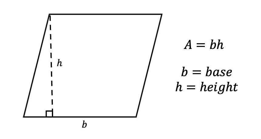
Why does the Formula for Area of a Parallelogram work?
Did you notice that the formula for area of a parallelogram above, base times height, is the same as the area formula for a rectangle? Why?
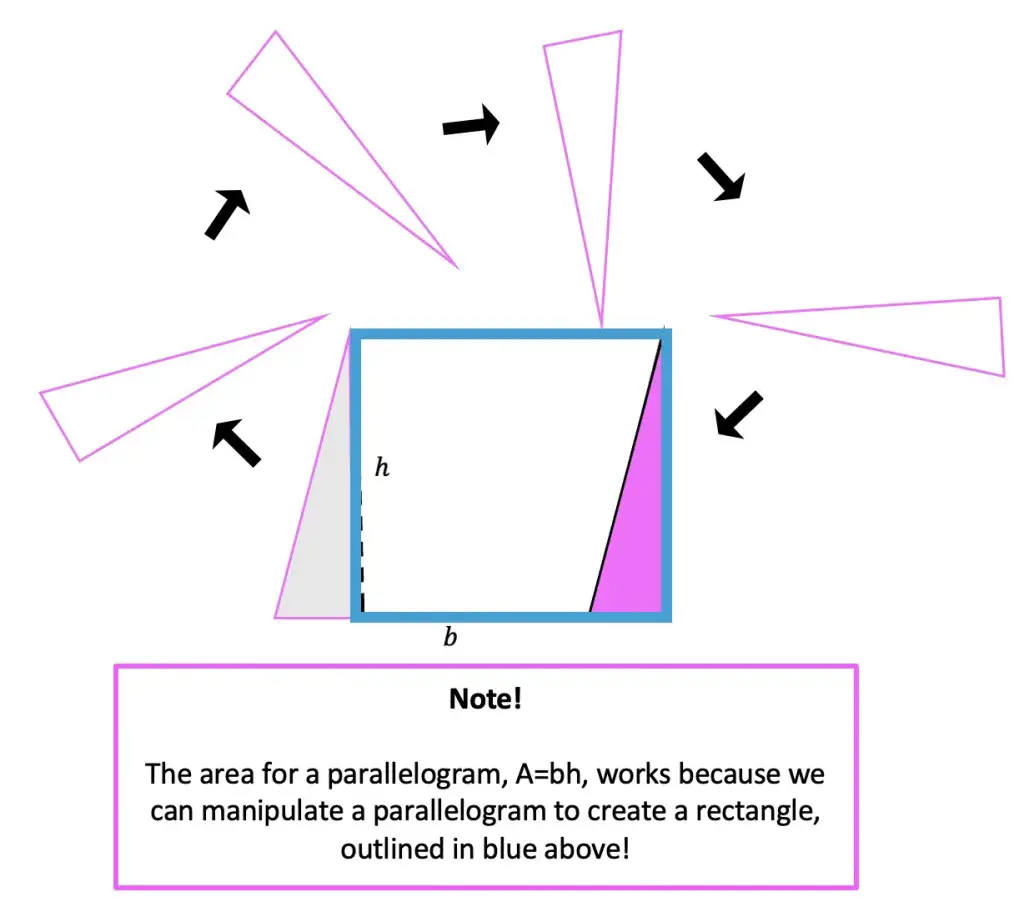
If we cut off the triangle that naturally forms along the dotted line of our parallelogram, rotated it, and placed it on the other side of our parallelogram, it would naturally fit like a puzzle piece and create a rectangle! Check it out below:
Now that we know where this formula comes from, let’s see it in action in the examples below:
Example #1:
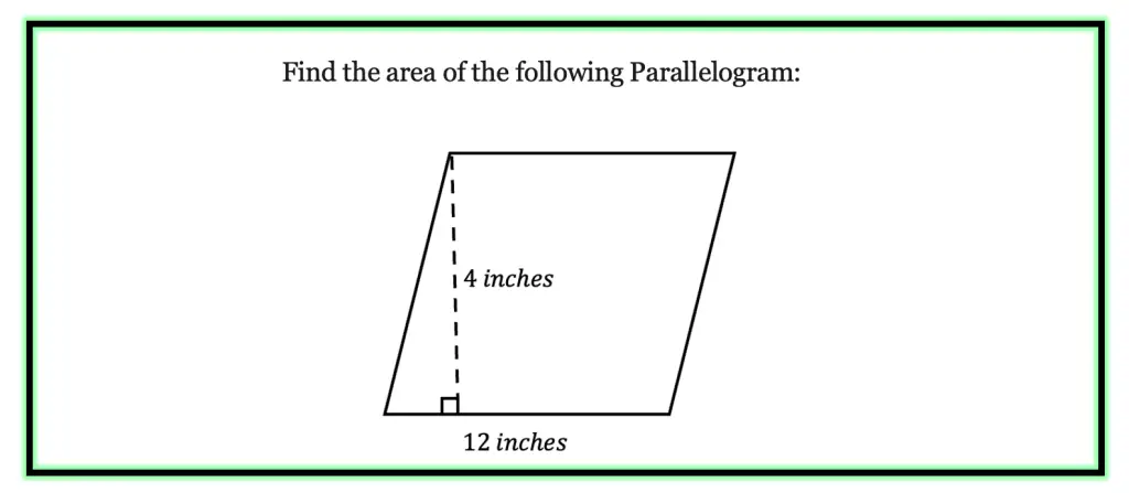
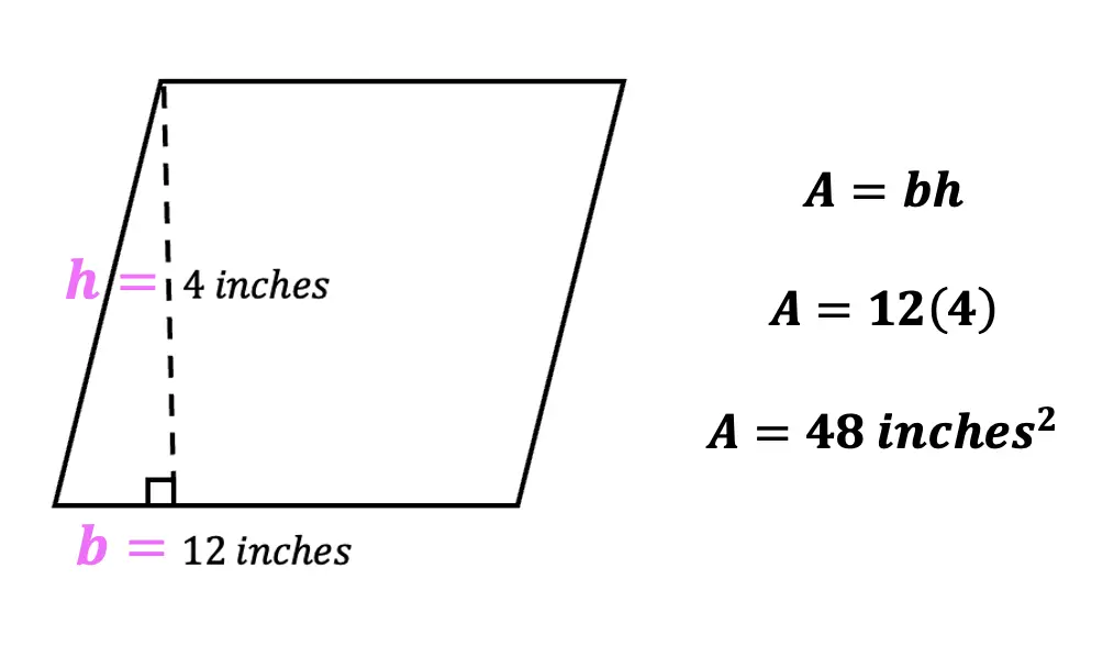
Step 1: Write out the formula:

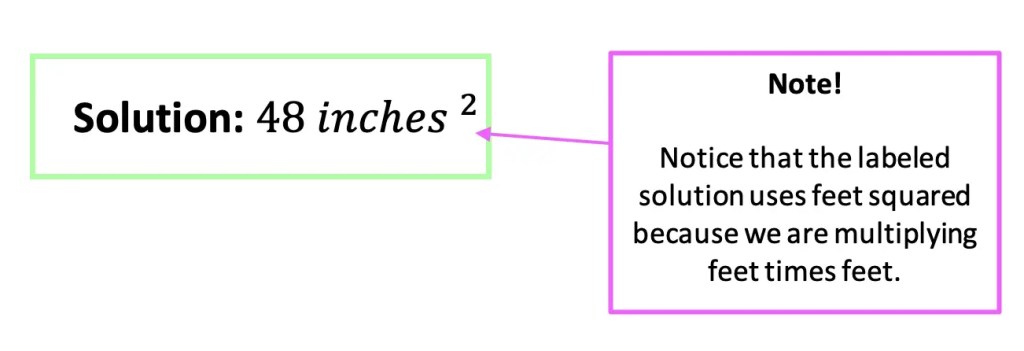
Step 2: Fill in the formula with values found on our parallelogram, b=12 inches h=4 inches, and multiply them together to get 48 inches squared.
That was a simple example, but lets try a harder one that involves special triangles.
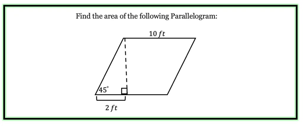
Example #2:
Step 1: Write out the formula:

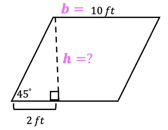
Step 2: Label the values found on our parallelogram, b=10 ft and notice that we are going to need to find the value of the height.
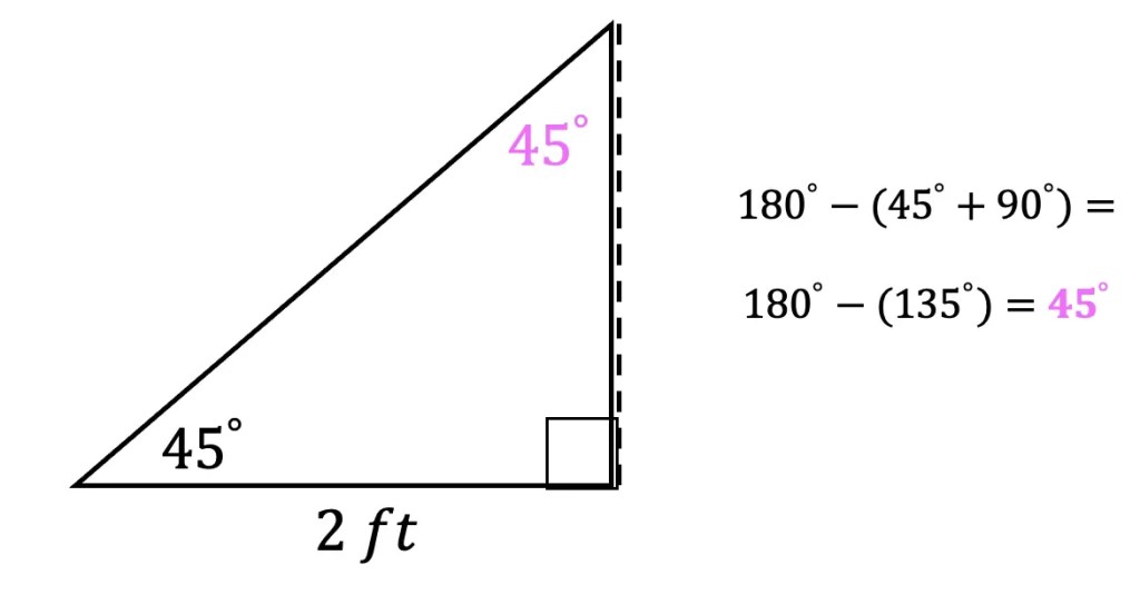
Step 3: In order to find the value of the height, we need to remember our special triangles! We are not given the value of the height, but we are given some value of the triangle that is formed by the dotted line. Let us take a closer look and expand this triangle:
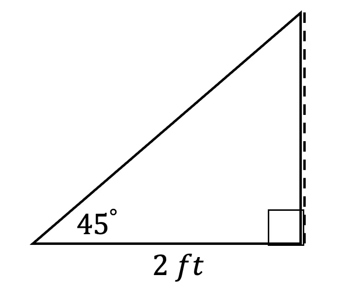
Step 4: We can add in the missing 45º degree value so that our triangle now sums to 180º.
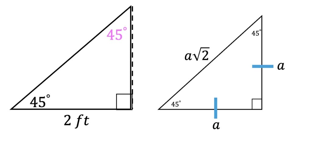
Step 5: Remember 45 45 90 special triangles? (If you need a review click the link). Because that is exactly what we are going to need to find the value of the height! Below is our triangle on the left, and on the right is the 45 45 90 triangle ratios we need to know to find the value of the height.
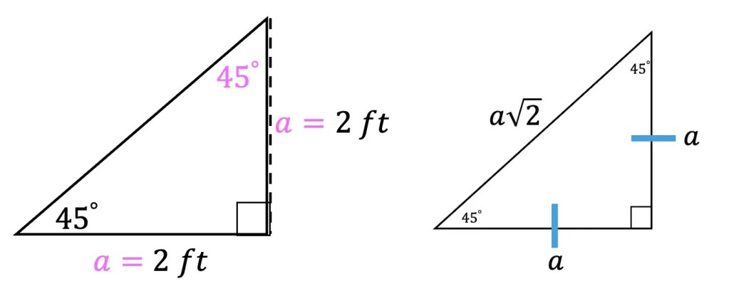
Based on the above ratios, we can figure out that the height value is the same value as the base of the triangle, 2.
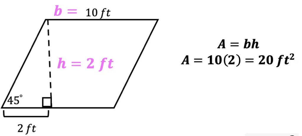
Step 6: If we place our triangle back into the original parallelogram, we can plug in our value for the height, h=2, into our formula to find the area:

When you’re ready, check out the practice questions below!
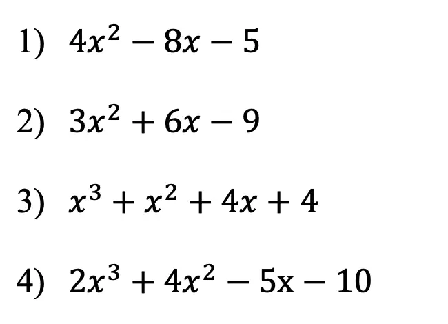
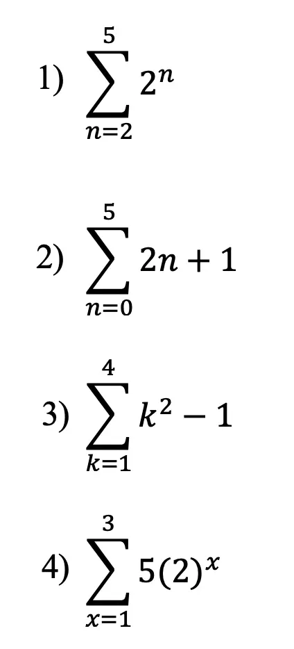
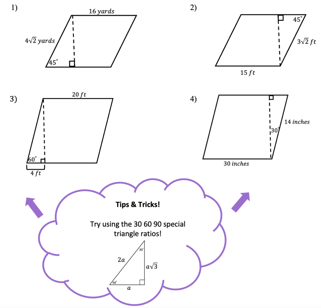
Practice Questions:
Find the area of each parallelogram:
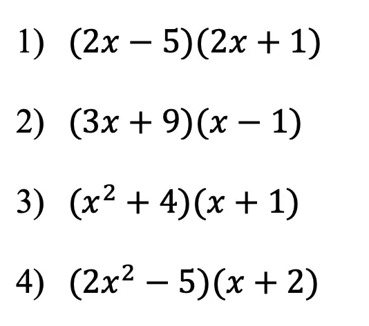
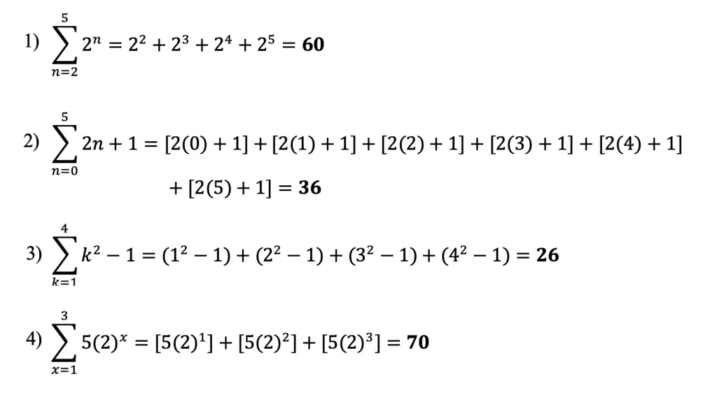
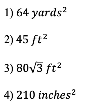
Solutions:
Still got questions? No problem! Don’t hesitate to comment with any questions or check out the video above. Happy calculating! 🙂
Facebook ~ Twitter ~ TikTok ~ Youtube