Hi everyone and welcome to MathSux! In today’s post we are going to be solving quadratic equations by using the quadratic formula. You may have used the quadratic formula before, but this time we are working with quadratic equations with two imaginary solutions. All this means is that there are negative numbers under the radical that have to be converted into imaginary numbers. If you need a review on imaginary numbers or the quadratic formula before reading this post, check out these links! Thanks so much for stopping by and happy calculating! 🙂
What is the Quadratic Formula?
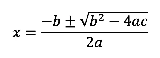
The Quadratic formula is a formula we use to find the x-values of a quadratic equation. When we find the x-value of a quadratic equation, we are actually finding its x-values on the coordinate plane. Check out the formula below:
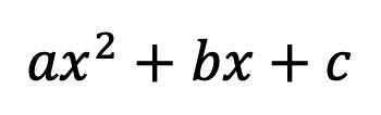
where, a, b, and c are coefficients based on the quadratic equation in standard form:
What does it mean to have “Imaginary Roots”?
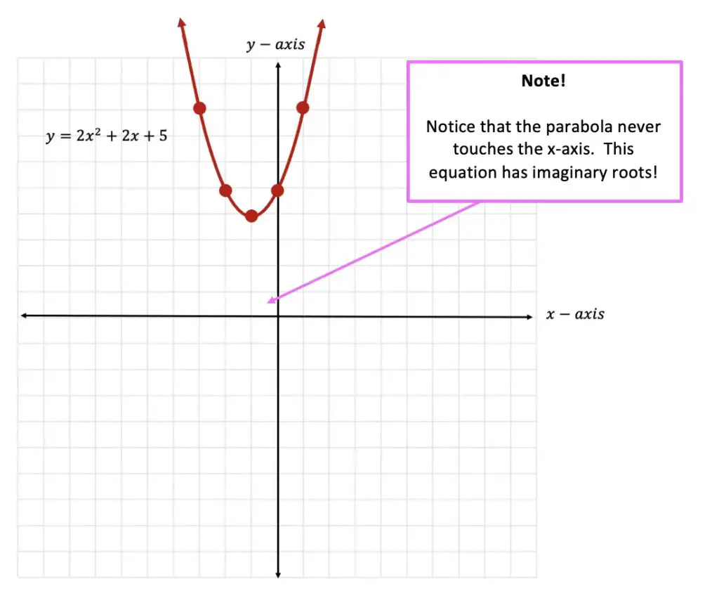
When we solve for the x-values of a quadratic equation, we are always looking for where the equation “hits” the x-axis. But when we have imaginary numbers as roots, the quadratic equation in question, never actually hit the x-axis. Ever. This creates a sort of “floating” quadratic equation with complex numbers as roots. See what it can look like below:
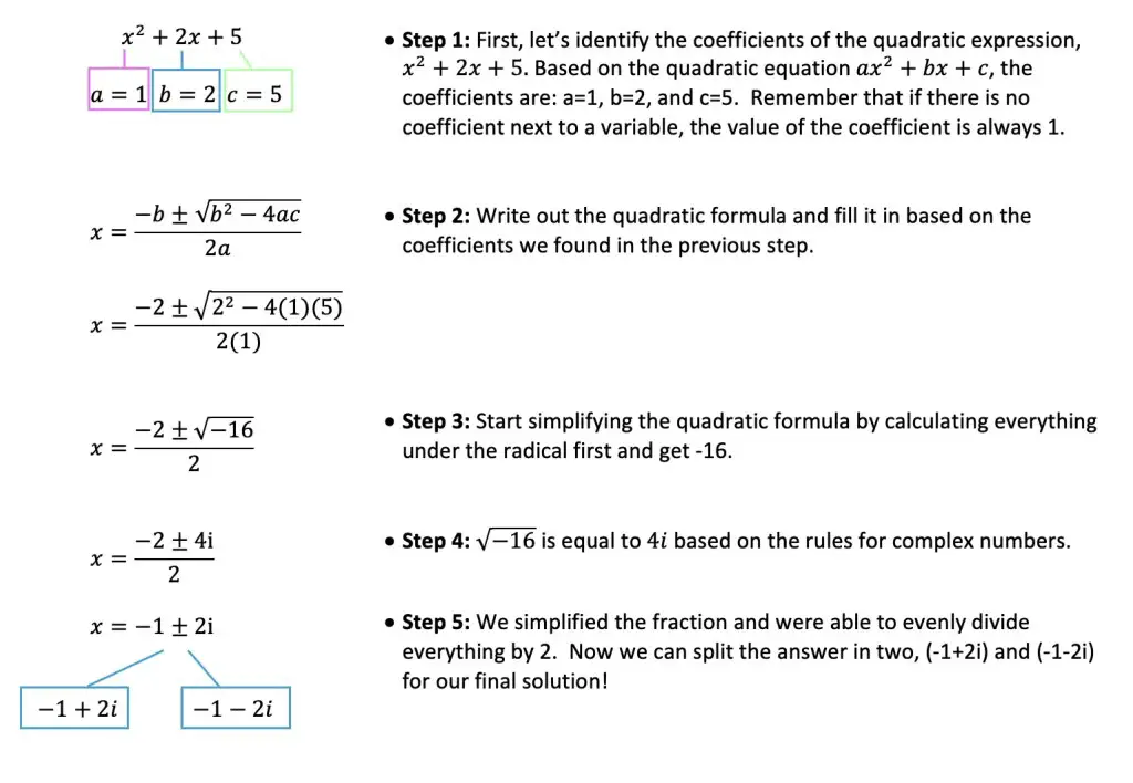
Ready for an Example? Let us see how to use the quadratic formula specifically, quadratic equations with two imaginary solutions:
Think you are ready to try practice questions on your own? Check out the ones below!
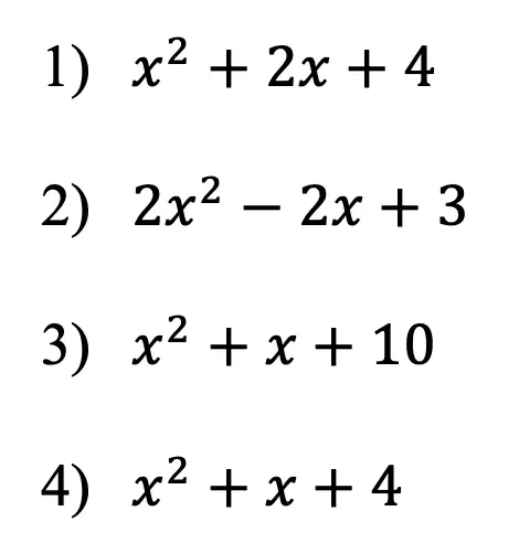
Practice Questions:
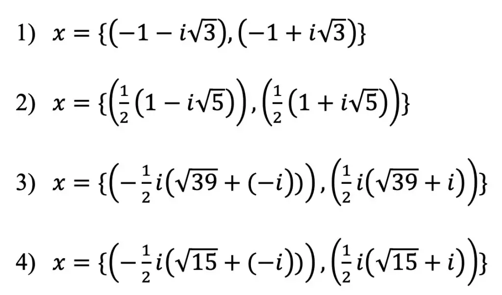
Solutions:
Still got questions? No problem! Don’t hesitate to comment with any questions below or check out the video above. Thanks for stopping by and happy calculating! 🙂
Hey there math peeps and welcome to MathSux! In today’s post we are going to cover factor by grouping examples, a surprisingly cool and easy factoring method used to factor quadratic equations when “a” is greater than one. It can also be used to factor four term polynomials. We are going to look at an example of each below. If you have any questions, please don’t hesitate to check out the video and try the practice problems at the end of this post. Thanks for stopping by and happy calculating! 🙂
What is Factor by Grouping?
Factor by Grouping is a factoring method that groups common factors of an algebraic expression together. Many times, we use factoring to find the x-values of a quadratic equation when the coefficient “a” is greater than 1.
When should we use Factor by Grouping?
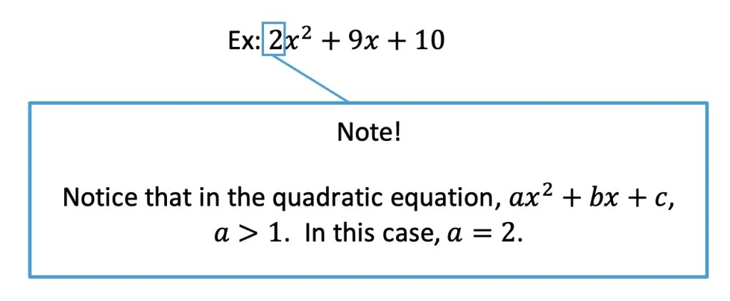
1) If the first coefficient in a quadratic equation, a, is greater than 1:
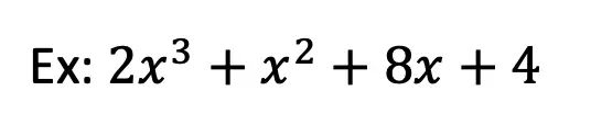
2) When there is a polynomial with 4 terms:
Factor by Grouping Examples:
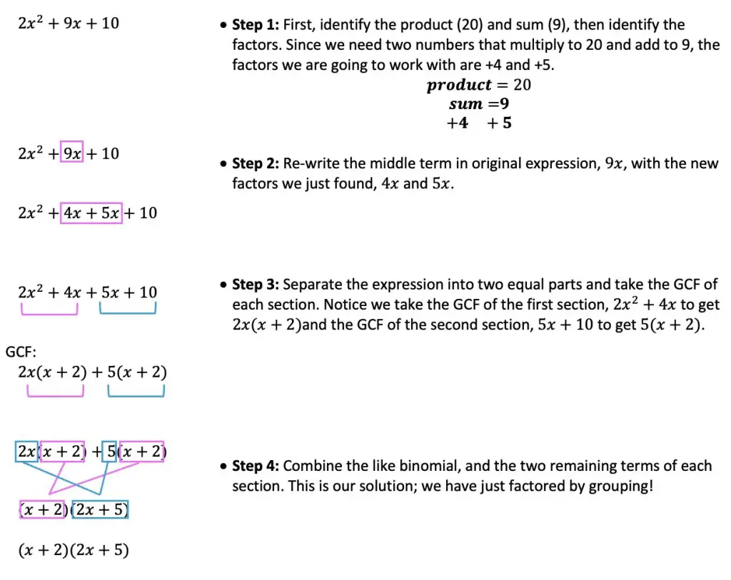
Ready for an Example? Let us look at how to factor a quadratic equation when a is greater than one.
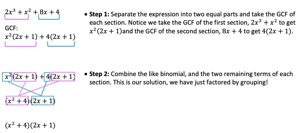
Now, let’s take a look at another type of example, that can be solved with the help of factor by grouping!
Notice that this question is actually easier to solve than the last! The polynomial above, is already split into 4 terms, therefore, we can jump ahead, skipping the product/sum steps we did in the previous example!
Ready to try practice questions on your own? Check them out below to master Factor by Grouping!
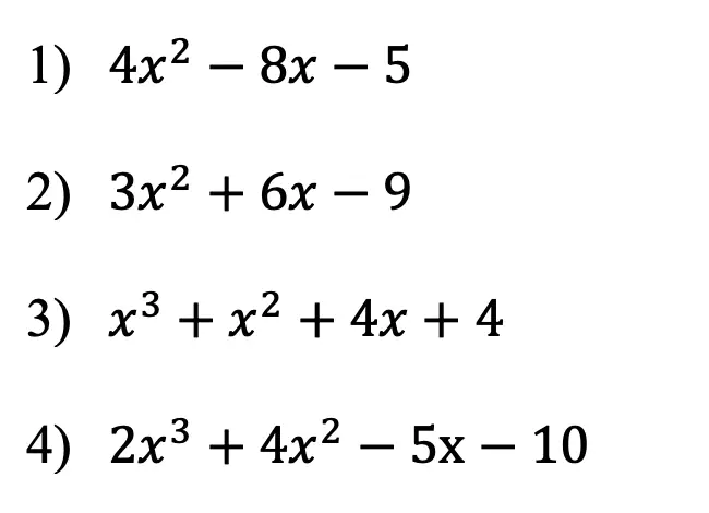
Practice Questions:
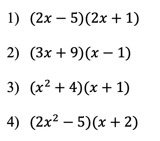
Solutions:
Still got questions? No problem! Don’t hesitate to comment with any questions below. Thanks for stopping by and happy calculating! 🙂
Hi everyone and happy Wednesday! Today we are going to look at how to solve inequalities with 2 variables. You may hear this in your class as “Simultaneous Inequalities” or “Systems of Inequalities,” all of these mean the same exact thing! The key to answering these types of questions, is to know how to graph inequalities and to know that the solution is always found where the two shaded regions overlap each other on the graph. We’re going to go over an example one step at time, then there will be practice questions at the end of this post that you can try on your own. Happy calculating! 🙂
How to Solve Inequalities with 2 Variables:
Just to review, when graphing linear inequalities, remember, we always want to treat the inequality as an equation of a line in form….with a few exceptions:
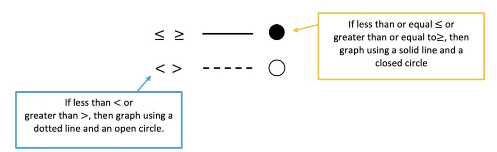
1)Depending on what type of inequality sign we are graphing, we will use either a dotted line and an open circle (< and >) or a solid line and a closed circle (> or <) and to correctly represent the solution.
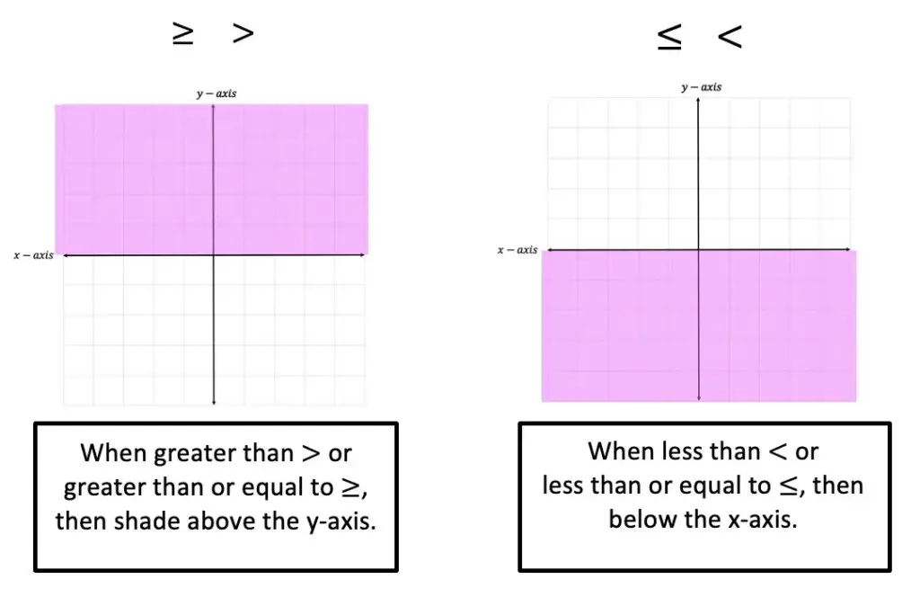
2) Shading is another important feature of graphing inequalities. Depending on the inequality sign we will need to either shade above the x-axis ( > or > ) or below the x-axis ( < or < ) to correctly represent the solution.
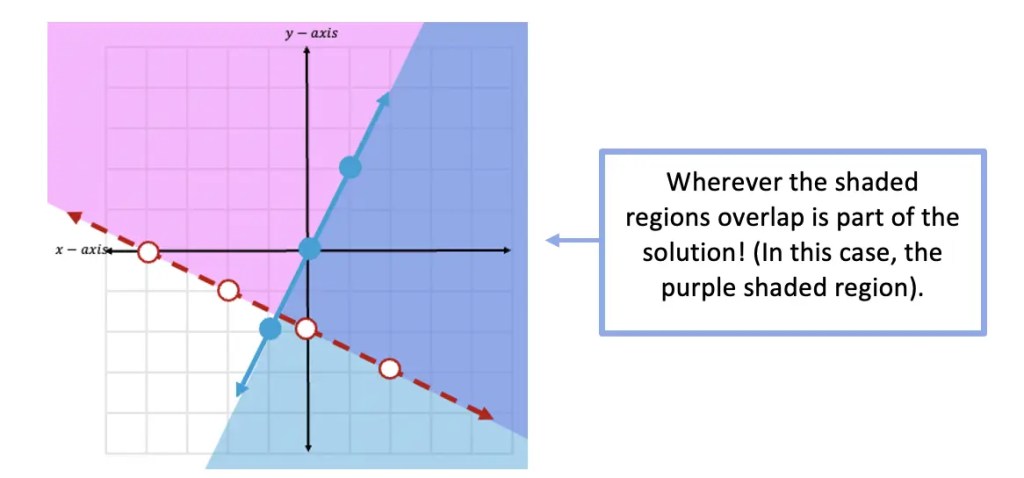
3) Solution: To find the solution of a system of inequalities, we are always going to look for where the shaded regions of both inequalities overlap.
Now that we know the rules, of graphing simultaneous inequalities, let’s take a look at an Example!
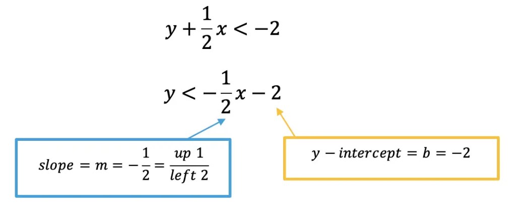
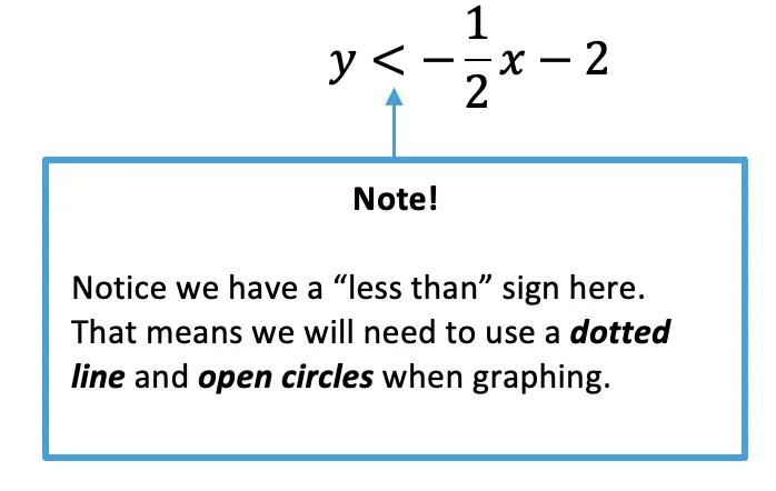
Step 1: First, let’s take our first inequality, and get it into y=mx+b form. To do this, we need to move .5x to the other side of the inequality by subtracting it from both sides. Once we do that, we can identify the slope and the y-intercept.
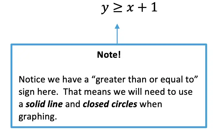
Step 2: Before graphing, let’s now identify what type of inequality we have here. Since we are working with a < sign, we will need to use a dotted lineand open circles when graphing.
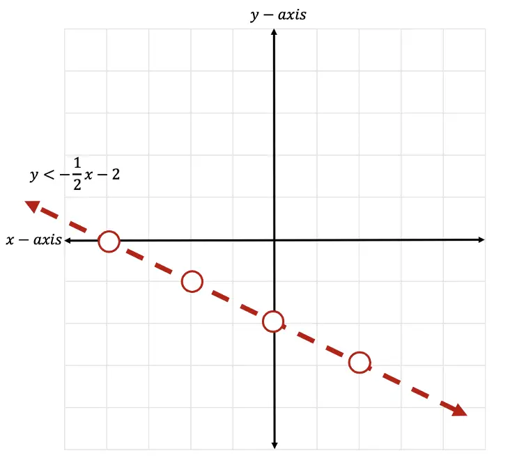
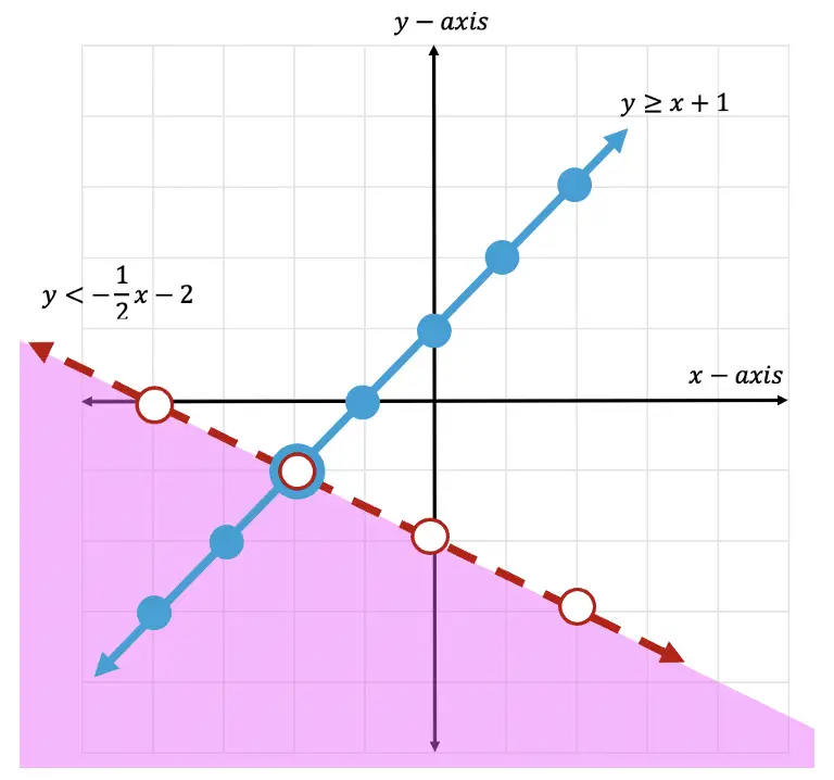
Step 3: Now that we have identified all the information we need to, let’s graph the first inequality below:
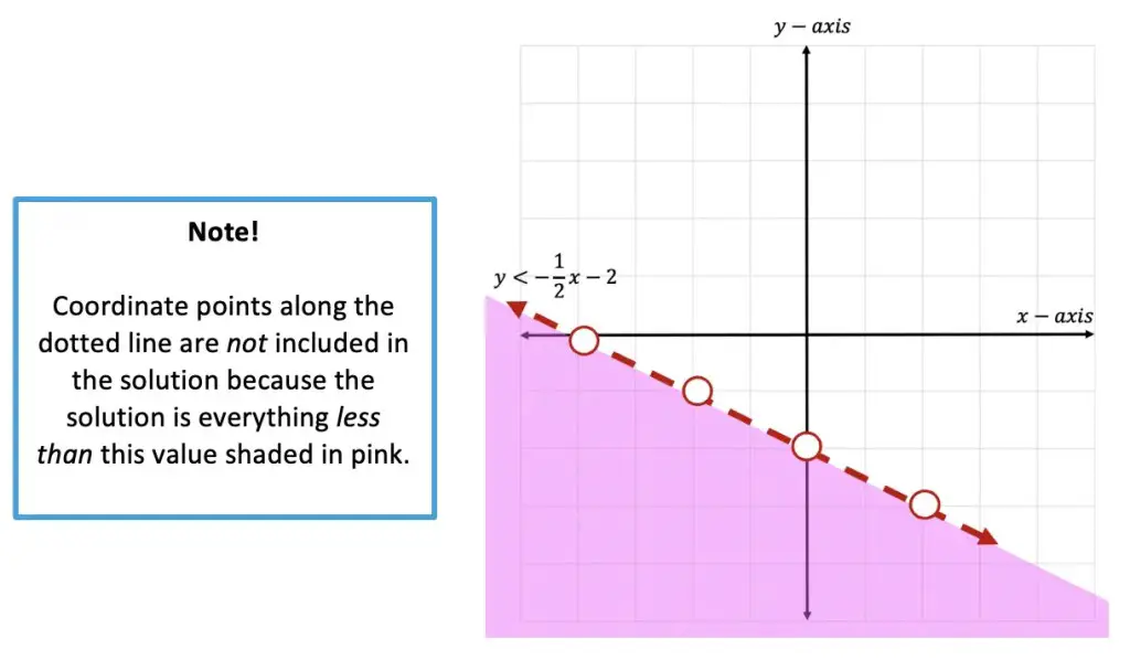
Step 4: Now it is time for us to shade our graph, since this is an inequality, we need to show all of our potential solutions with shading. Since we have a less than sign, <, we will be shading below the x-axis. Notice all the negative y-values below are included to the left of our line. This is where we will shade.
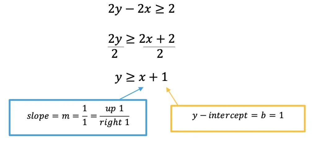
Step 5: Next, let’s start graphing our second inequality! We do this by taking the second equation, and getting it into y=mx+b form. To do this, we need to move 2x to the other side of the inequality by adding it to both sides. Then we can simplify the inequality even further by dividing out a 2.
Step 6: Before graphing, let’s now identify what type of inequality we have here. Since we are working with a > sign, we will need to use a solid lineand closed circles when creating our graph.
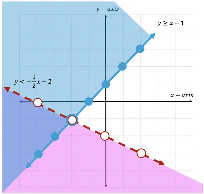
Step 7: Now that we have identified all the information we need to, let’s graph the second inequality below:
Step 8: Now it is time for us to shade our graph. Since we have a greater than or equal to sign, >, we will be shading above the x-axis. Notice all the positive y-values above are included to the left of our line. This is where we will shade.
Where is the solution?!
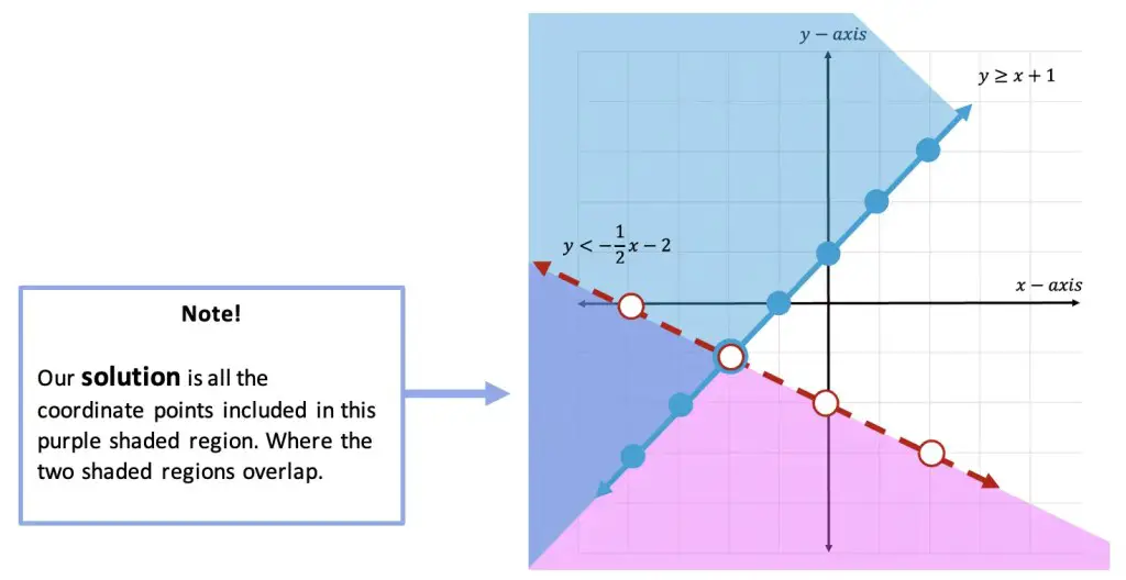
Step 9: The solution is found where the two shaded regions overlap. In this case, we can see that the two shaded regions overlap in the purple section of this graph.
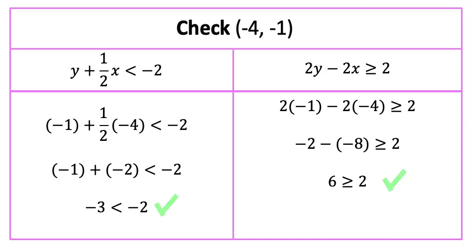
Step 10: Check! Now we can finally check our work. To do that, we can choose any point within our overlapping purple shaded region, if the coordinate point we choose holds true when plugged into both of our inequalities then our graph is correct!
Let’s take the point (-4,-1) and plug it into both original inequalities where x=-4 and y=-1.
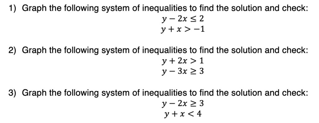
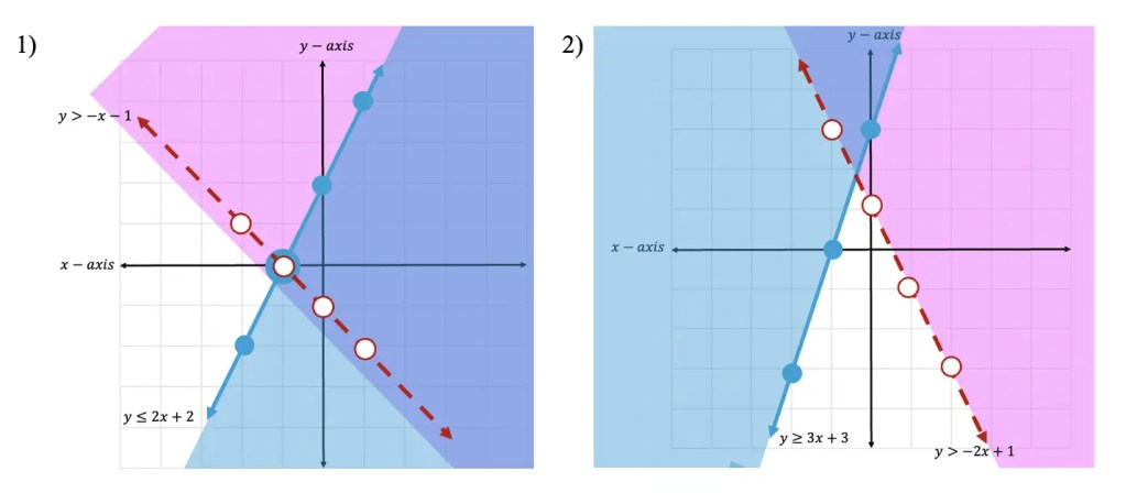
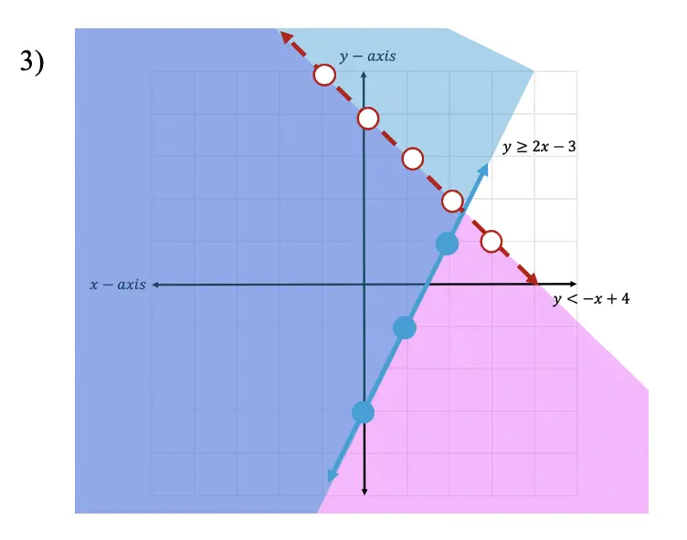
Practice Questions:
Solutions:
Still got questions? No problem! Don’t hesitate to comment with any questions below. Thanks for stopping by and happy calculating! 🙂
Hi everyone and welcome to MathSux! In this post we are going to go over summation notation (aka sigma notation). The summing of a series isn’t hard as long as you know how to read the notation! We will go over an example and breakdown what each part of this notation represents step by step. When you are ready, please don’t forget to check out the practice questions at the end of this post to truly master the topic. Thanks for stopping by and happy calculating! 🙂
What is Summation Notation?
Summationnotation lets us write a series in an easy and short-handed way. Before we go any further we also need to define a series!
Series: The sum of adding each term within an infinite sequence. This can include arithmetic or geometric sequences we are already familiar with. For example, let’s say we have the arithmetic sequence: 2,4,6,8, ….. now with a series we are adding all of these terms together: 2+4+6+8+……
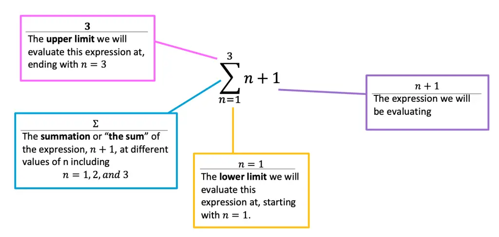
Now back to summations. Summations allow us to quickly understand that the sequence being added together is done so on an infinite or finite basis by giving us a range of values for which the unknown variable can be evaluated and summed together. Summation notation is represented with the capital Greek letter sigma, Σ, with numbers below and above as limits for calculation and the series that must be evaluated to the right.
If this sounds confusing, don’t worry, it might sound more confusing than it actually is! Take a look at the breakdown for sigma notation below:
Wait, what does the above summation say?
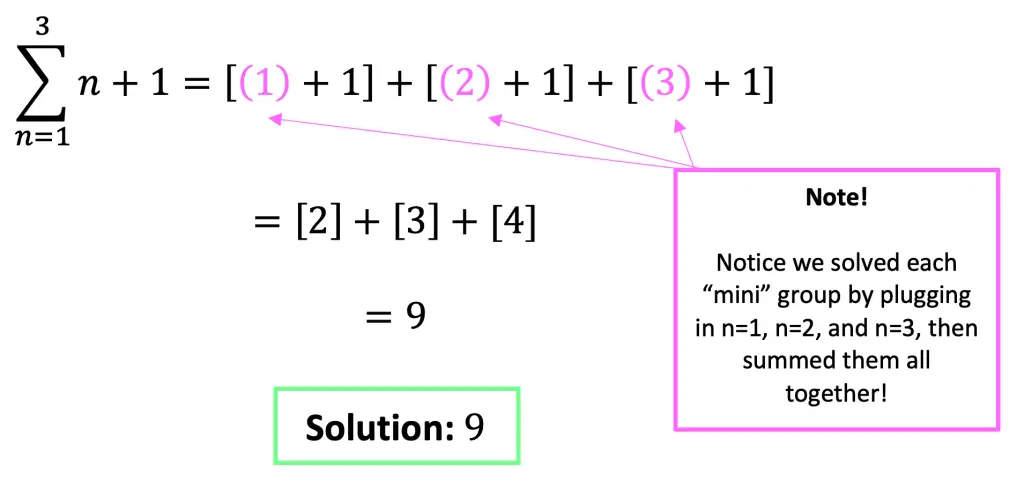
Translation: It tells us to evaluate the expression, n+1 by plugging in 1 for n, 2 for n, and 3 for n and then wants us to sum all three solutions together.
Take a look below to see how to solve this step by step:
Check out the video above to see more examples step by step! When you’re ready to try them on your own, check out the practice problems below:
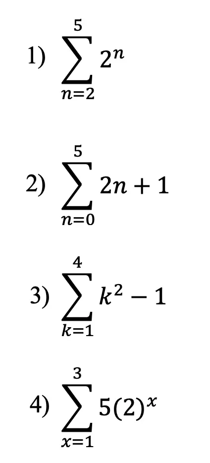
Practice Questions:
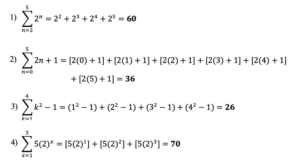
Solutions:
Still got questions? No problem! Don’t hesitate to comment with any questions below. Thanks for stopping by and happy calculating! 🙂
Looking for something similar to sigma notation? Check out this post on geometric sequences here! If you’re looking for more statistics formulas, check out how to find expected value!
Greeting math friends and welcome to MathSux! In today’s post we are going to review and take a look at how to use the graphing calculator available by the French company, NumWorks.
In this NumWorks calculator review, first impressions are that this is a serious competitor for Texas Instruments and offers more features than a typical calculator with a focus on statistics, data analysis, and even computer programming! Check out the video below to see the un-boxing, full review, and how to use this calculator step by step. Happy calculating! 🙂
NumWorks Calculator Stand Out Features:
1) TheHome Screen: Works and looks like apps on an iPhone. It is super easy to use, and includes apps such as the regular graphing calculator we’re all used to, as well as, Python, Statistics, Probability, Equation Solver, Sequences, and Regression.
2) The Equation Solver: Punch in any function and find it’s x-values and discriminant! Very cool!
3) Python: Yes, this calculator is programmable via Python! It also includes pre-made scripts that you can easily run. This is great for aspiring programmers and important for today’s economy.
4) Exam Mode: Teachers can make students put their calculators in exam mode and watch their students calculators light up in red to prove there’s no cheating funny business going on! Warning though, this will delete all of your data including the pre-made Python scripts. But you can always hit the reset button in the back to reset.
Did I mention math teacher’s can potentially get a free calculator from NumWorks? Check out the link here!
Has anyone else tried this graphing calculator from NumWorks? What were your first thoughts? Let me know in the comments and happy calculating!
Happy new year and welcome to Math Sux! In this post we are going to dive right into simultaneous equations and how to solve them three different ways! We will go over how to solve simultaneous equations using the (1) Substitution Method (2) Elimination Method and (3) Graphing Method. Each and every method leading us to the same exact answer! At the end of this post don’t forget to try the practice questions choosing the method that best works for you! Happy calculating! 🙂
What are Simultaneous Equations?
Simultaneous Equations are when two equations are graphed on a coordinate plane and they intersect at, at least one point. The coordinate point of intersection for both equation is the answer we are trying to find when solving for simultaneous equations. There are three different methods for finding this answer:
We’re going to go over each method for solving simultaneous equations step by step with the example below:
Method #1: Substitution
The idea behind Substitution, is to solve for 1 variable first algebraically, and the plug this value back into the other equation solving for one variable. Then solving for the remaining variable. If this sounds confusing, don’t worry! We’re going to do this step by step:
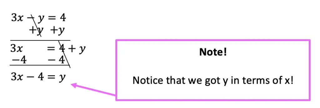
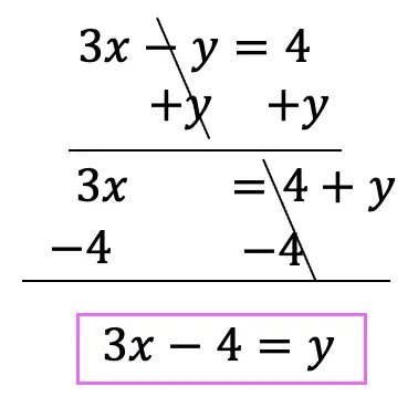
Step 1: Let’s choose the first equation and move our terms around to solve for y.
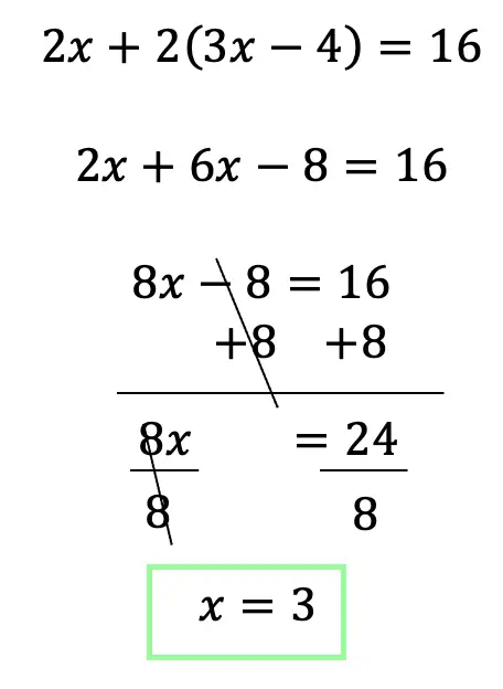
Step 3: The equation is set up and ready to solve for x!
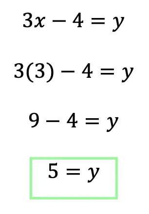
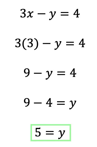
Step 4: All we need to do now, is plug x=3 into one of our original equations to solve for y.
Step 5: Now that we have solved for both x and y, we have officially found where these two simultaneous equations meet!
Method #2: Elimination
The main idea of Elimination is to add our two equations together to cancel out one of the variables, allowing us to solve for the remaining variable. We do this by lining up both equations one on top of the other and adding them together. If variables at first do not easily cancel out, we then multiply one of the equations by a number so it can. Check out how it’s done step by step below!
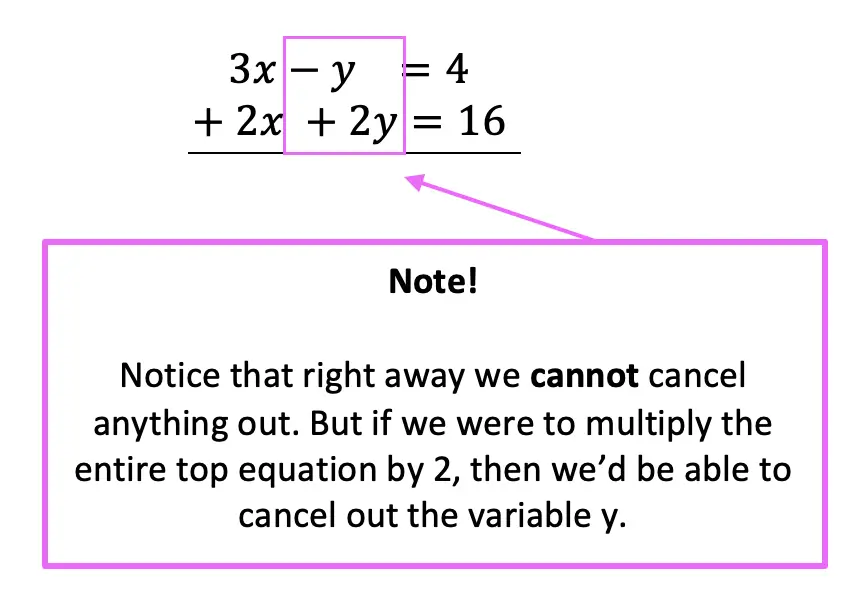
Step 1: First, let’s stack both equations one on top of the other to see if we can cancel anything out:
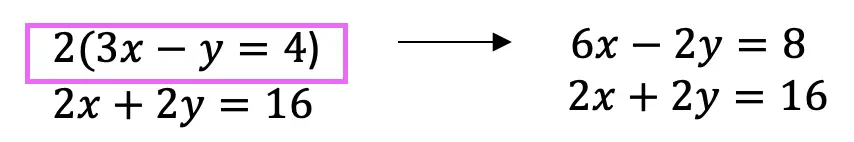
Step 2: Our goal is to get a 2 in front of y in the first equation, so we are going to multiply the entire first equation by 2.
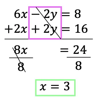
Step 3: Now that we multiplied the entire first equation by 2, we can line up our two equations again, adding them together, this time canceling out the variable y to solve for x.
Step 4: Now, that we’ve found the value of variable x=3, we can plug this into one of our equations and solve for missing unknown variable y.
Step 5: Now that we have solved for both x and y, we have officially found where these two simultaneous equations meet!
Method #3: Graphing
The main idea of Graphing is to graph each a equation on a coordinate plane and then see at what point they intersect. This is the best method to visualize and check our answer!
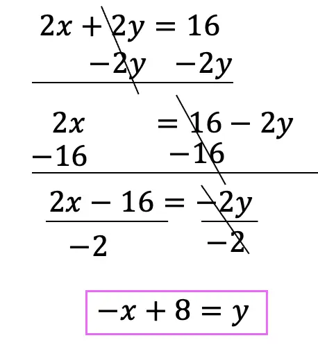
Step 1: Before we start graphing let’s convert each equation into y=mx+b (equation of a line) form.
Equation 1:
Equation 2:
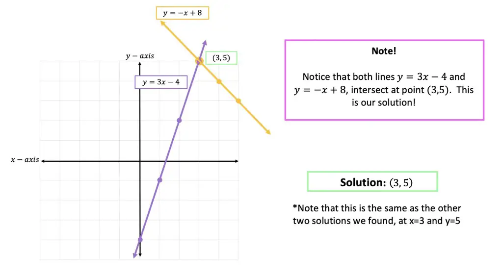
Step 2: Now, let’s graph each line, y=3x-4 and y=-x+8, to see at what coordinate point they intersect.
Need to review how to draw an equation of a line? Check out this post here! Notice we got the same exact answer using all three methods (1) Substitution (2) Elimination and (3) Graphing.
Ready to try the practice problems on your own?! Check them out below!
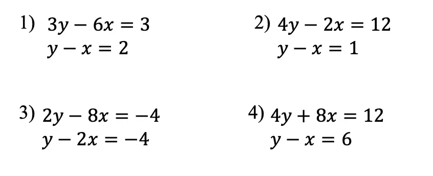
Practice Questions:
Solve the following simultaneous equations for x and y.
Solutions:
(1, 3)
(4,5)
(-1, -6)
(3, -3)
Want more MathSux? Don’t forget to check out our Youtube channel and more below! And if you have any questions, please don’t hesitate to comment below. Happy Calculating!
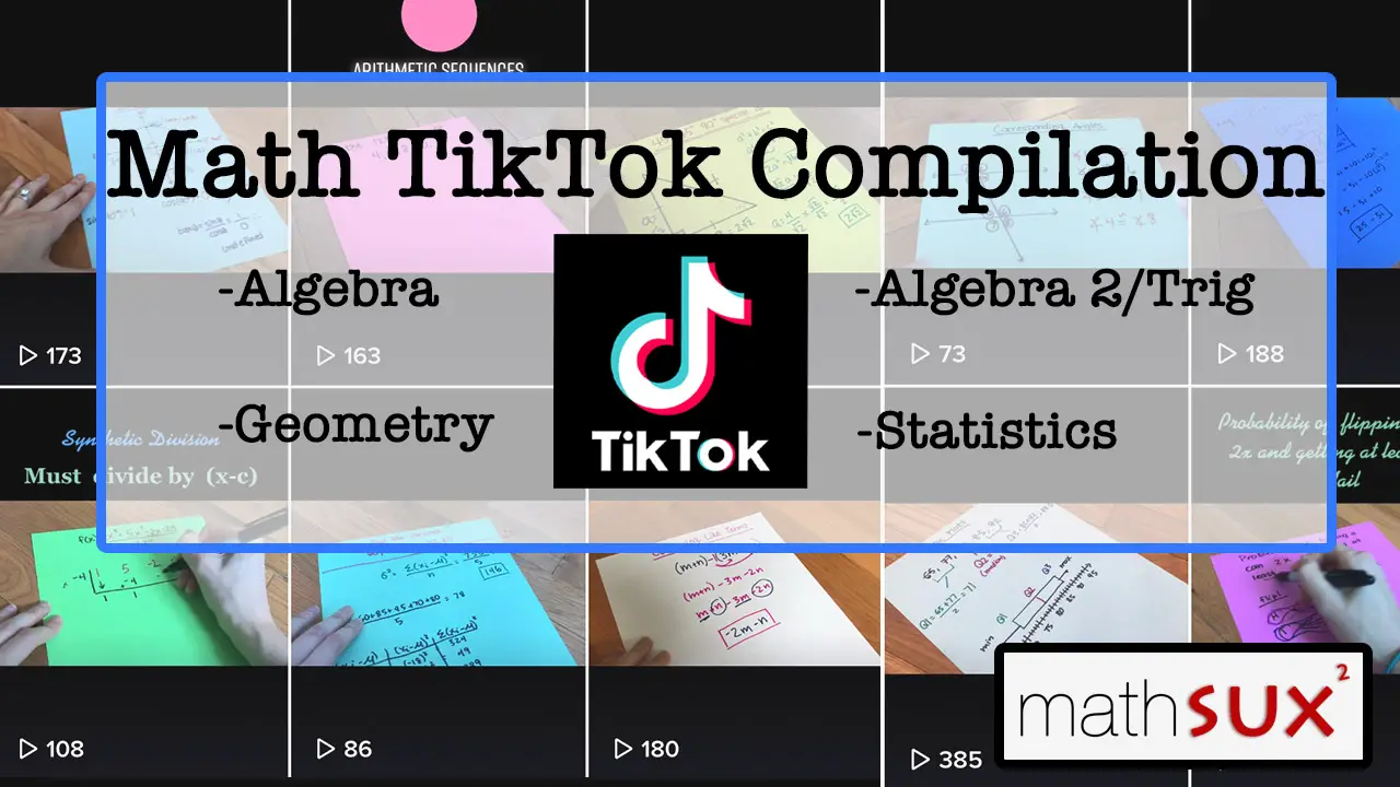
Happy December everyone! With crazy 2020 coming to an end, I thought I would share some TikTok math video compilations of Algebra, Geometry, Algebra 2/Trig, and Statistics for a quick review of all our videos posted throughout the year. Enjoy these TikTok math video compilations and happy calculating! 🙂
Want to make math suck just a little bit less? Subscribe and follow us for FREE fun colorful math videos and lessons every week! 🙂
Within algebra, you will find arithmetic sequences, combining like terms, box and whisker plots, geometric sequences, solving radical equations, completing the square, 4 ways to factor quadratic equations, piecewise functions and more!
Geometry:
Within Geometry, you will find, how to construct an equilateral triangle, a median of a trapezoid, area of a sector, how to find perpendicular and parallel lines through a given point, SOH CAH TOA right triangle trigonometry, reflections, and more!
Algebra 2/Trig.
Within Algebra 2/Trig., you will find, how to expand a cubed binomial, how to divide polynomials, how to solve log equations, imaginary numbers, synthetic division, unit circle basics, how to graph y=sin(x), and more!
Statistics:
Within statistics, you will find, box and whisker plots, how to find the variance, and, the probability of flipping a coin 2 times!
For full length video, don’t forget to check out our free math video index page! Thanks for stopping by! 🙂
r=Common Ratio (Number Multiplied/Divided by each successive term in sequence)
n= Term Number in Sequence
Hi everyone and welcome to Mathsux! In this post, we are going to answer the question, what is a geometric sequence (otherwise known as a geometric progression)? We will accomplish this by learning how to identify a geometric sequence, then we will break down the geometric sequence formula an=a1r(n-1), and solve two different types of examples. As always if you want more questions, check out the video below and the practice problems at the end of this post. Happy calculating! 🙂
What are Geometric Sequences?
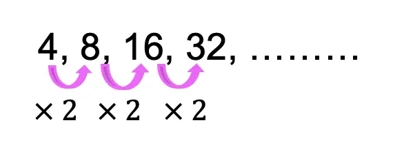
Geometric sequences are a sequence of numbers that form a pattern when the same number is either multiplied or divided to each subsequent term. Take a look at the example of a geometric sequence below:
Example:
Notice we are multiplying 2 by each term in the sequence above. If the pattern were to continue, the next term of the sequence above would be 64. This is a geometric sequence!
In this geometric sequence, it is easy for us to see what the next term is, but what if we wanted to know the 15th term? Instead of writing out and multiplying our terms 15 times, we can use a shortcut, and that’s where the Geometric Sequence formula comes in handy!
Geometric Sequence Formula:
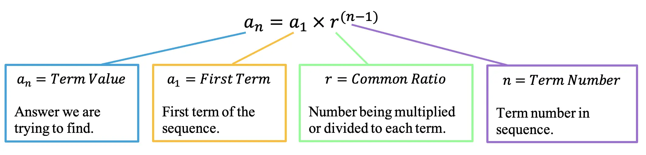
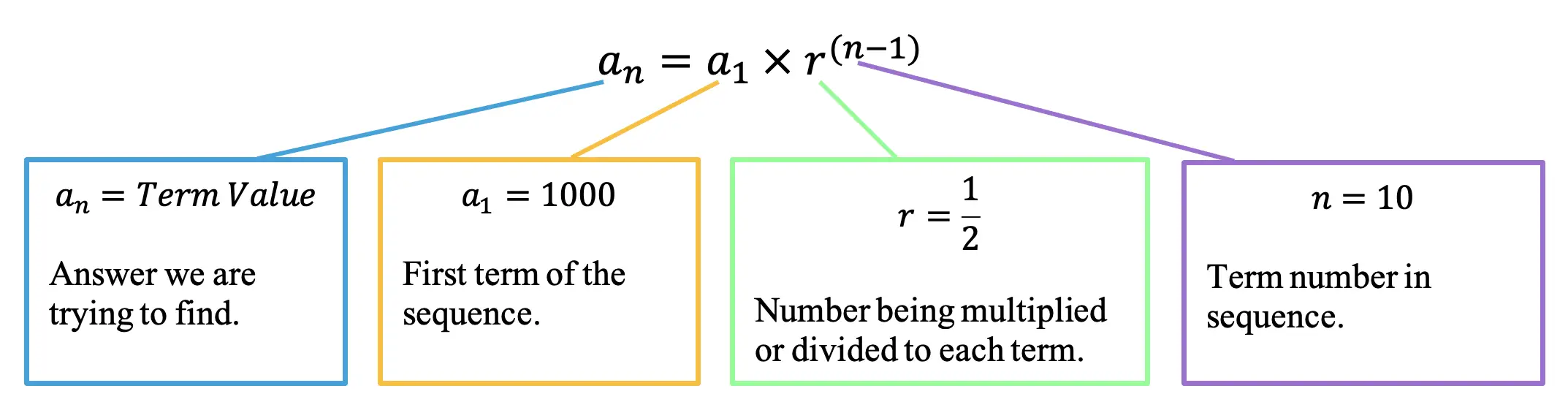
Take a look at the geometric sequence formula below, where each piece of our formula is identified with a purpose.
an=a1r(n-1)
a1 = The first term is always going to be that initial term that starts our geometric sequence. In this case, our sequence is 4,8,16,32, …… so our first term is the number 4.
r= One key thing to notice about the formula below that is unique to geometric sequences is something called the Common Ratio. The common ratio is the number that is multiplied or divided to each consecutive term within the sequence.
n= Another interesting piece of our formula is the letter n, this always stands for the term number we are trying to find. A great way to remember this is by thinking of the term we are trying to find as the nthterm, which is unknown.
Now that we broke down our geometric sequence formula, let’s try to answer our original question below:
Example #1: Common ratio r>1
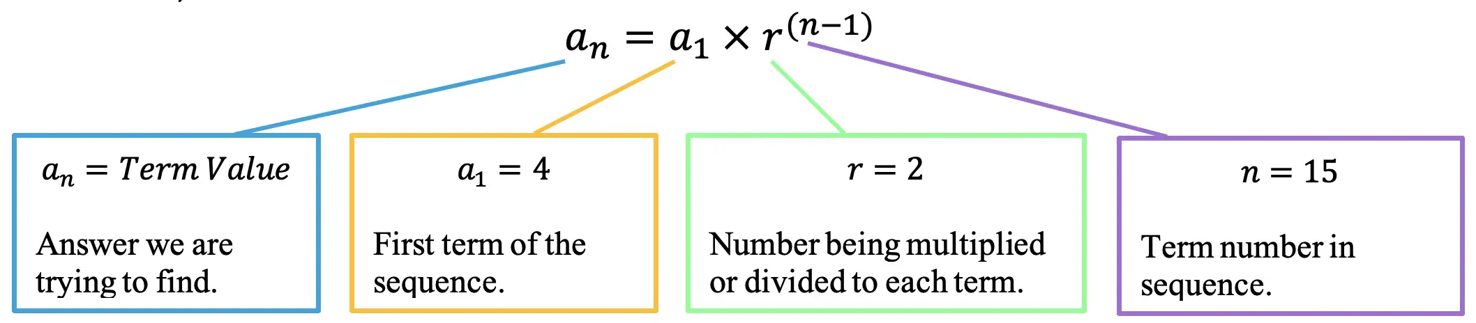
Step 1: First let’s identify the common ratio between each previous and subsequent term of the sequence. Notice each term in the sequence is multiplied by 2 (as we identified earlier in this post). Therefore, our common ratio for this sequence is 2.
Step 2: Next, let’s write the geometric sequence formula and identify each part of our formula (First Term=4, Term number=15, common ratio=2).
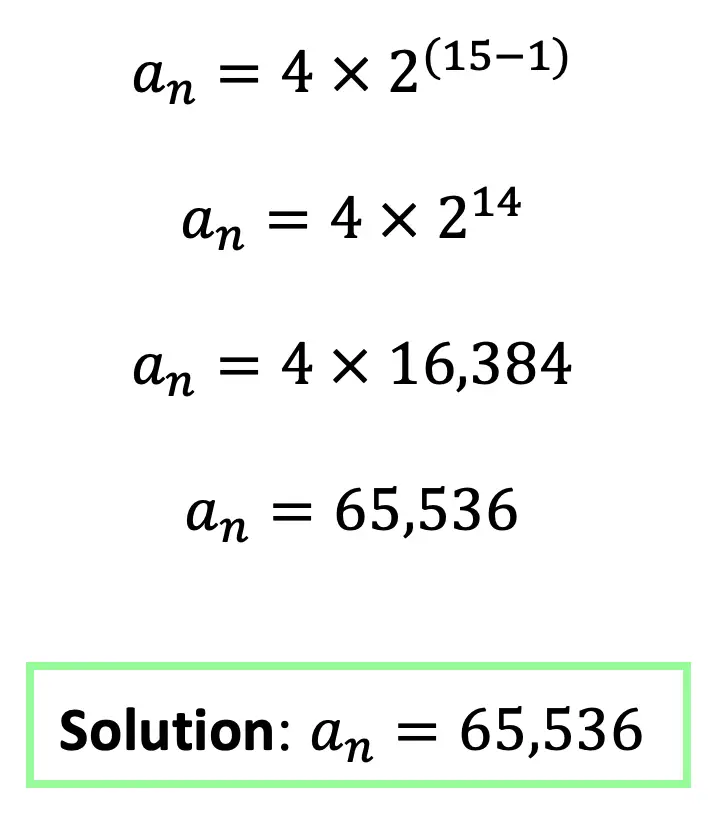
Step 3: Now let’s fill in our formula and solve with the given values.
Let’s look at another example where, the common ratio is a bit different, and instead of multiplying a number, this time we are going to be dividing the same number from each subsequent term, (this can also be thought of as multiplying by a common ratio that is a fraction):
Example #2: Common ratio 0<r<1
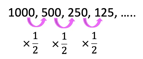
Step 1: First let’s identify the common ratio between each number in the sequence. Notice each term in the sequence is divided by 2 (or multiplied by 1/2 that way it is shown below).
Step 2: Next, let’s write the geometric sequence formula and identify each part of our formula (First Term=1000, Term number=10, common ratio=1/2).
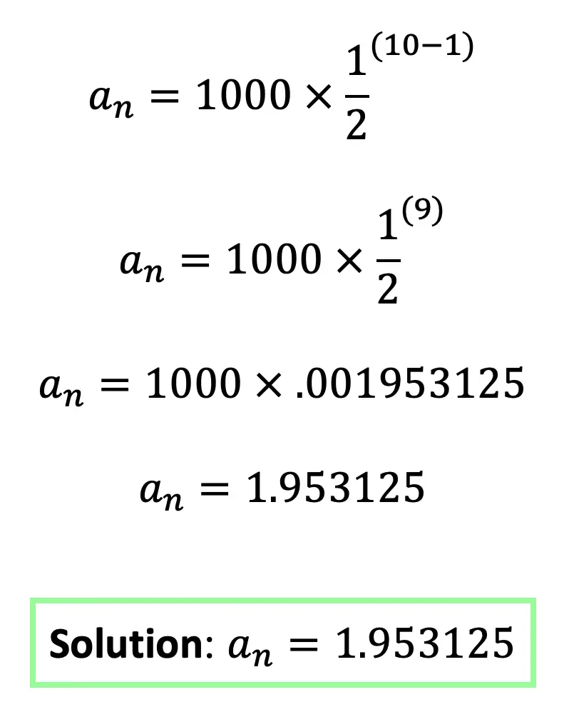
Step 3: Next let’s fill in our formula and solve with the given values.
Think you are ready to practice solving geometric sequences on your own? Try the following practice questions with solutions below:
Practice Questions:
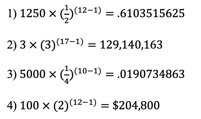
Find the 12th term given the following sequence: 1250, 625, 312.5, 156.25, 78.125, ….
Find the 17th term given the following sequence: 3, 9, 27, 81, 243,…..
Find the 10th term given the geometric sequence: 5000, 1250, 312.5, 78.125 …..
Shirley has $100 that she deposits in the bank. She continues to deposit twice the amount of money every month. How much money will she deposit in the twelfth month at the end of the year?
Solutions:
Fun Fact!
Did you know that the geometric sequence formula can be considered an explicit formula? An explicit formula means that even though we do not know the other terms of a sequence, we can still find the unknown value of any term within the given sequence. For example, in the first example we did in this post (example #1), we wanted to find the value of the 15th term of the sequence. We were able to do this by using the explicit geometric sequence formula, and most importantly, we were able to do this without finding the first 14 previous terms one by one…life is so much easier when there is an explicit geometric sequence formula in your life!
Other examples of explicit formulas can be found within the arithmetic sequence formula and the harmonic series.
Related Posts:
Looking to learn more about sequences? You’ve come to the right place! Check out these sequence resources and posts below. Personally, I recommend looking at the finite geometric sequence or infinite geometric series posts next!
Still, got questions? No problem! Don’t hesitate to comment below or reach out via email. And if you would like to see more MathSux content, please help support us by following ad subscribing to one of our platforms. Thanks so much for stopping by and happy calculating!
d=Common Difference (Number Added/Subtracted to each Term in Sequence)
Hi everyone and welcome to Mathsux! In this post, we’re going to go over arithmetic sequences (otherwise known as arithmetic progression). We’ll identify what arithmetic sequences are, break down each part of the arithmetic sequence formula an=a1+(n-1)d, and solve two different types of examples. As always if you want more questions, check out the video below and the practice problems at the end of this post. Happy calculating! 🙂
What are Arithmetic Sequences?
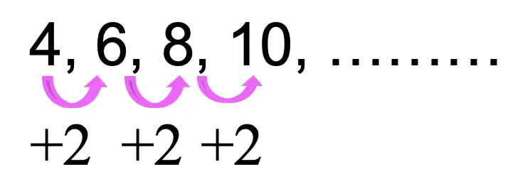
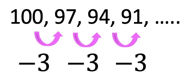
Arithmetic sequences are a sequence of numbers that form a pattern when the same number is either added or subtracted to each successive term. Take a look at the example of an arithmetic sequence below:
Notice the pattern? We are adding the number 2 to each term in the sequence above. If the pattern were to continue, the next term of the sequence above would be 10+2 which gives us 12. This is an arithmetic sequence!
In the above sequence, it’s easy for us to identify what the next term in the sequence would be, but what happens if we were asked to find the 123rd term of an arithmetic sequence? That’s where the Arithmetic Sequence Formula would come in handy!
Arithmetic Sequence Formula:
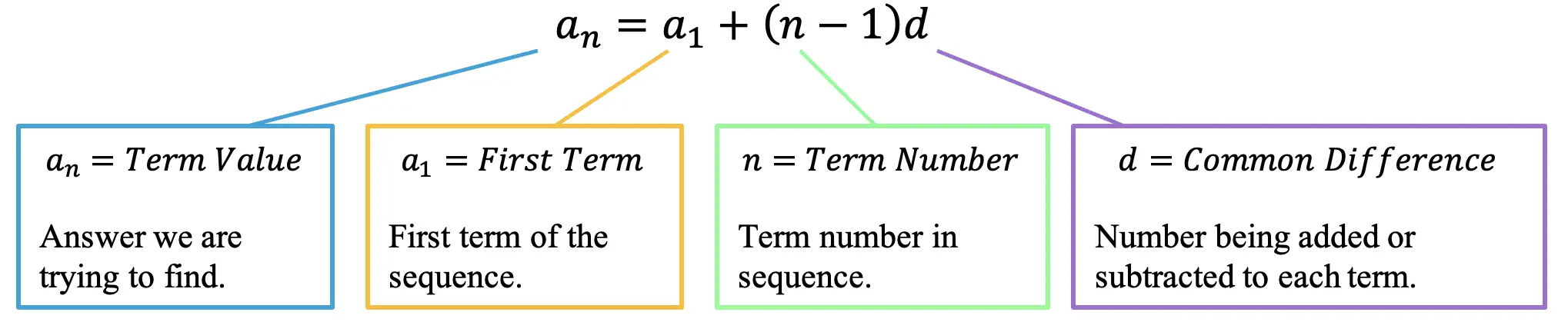
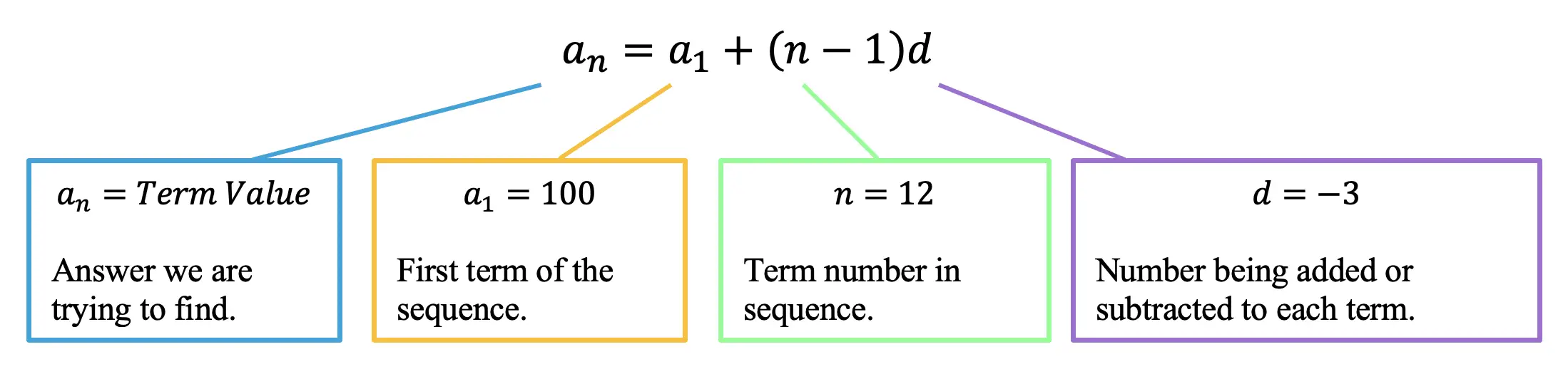
Take a look at the arithmetic sequence formula below, where each piece of our formula is identified with a purpose.
an=a1+(n-1)d
a1= The first term is always going to be that initial term that starts our arithmetic sequence. In this case, our sequence is 4,6,8,10, …… so our first term is the number 4.
n= Another interesting piece of our formula is the letter n, this always stands for the term number we are trying to find. A great way to remember this is by thinking of the term we are trying to find as the nthterm, which is unknown.
d = One key thing to notice about the formula below that is unique to arithmetic sequences is something called the Common Difference. The common difference is the number that is added or subtracted to each consecutive term within the sequence.
Now that we know the arithmetic sequence formula, let’s try to answer our original question below:
Step 1: First let’s identify the common difference between each previous and subsequent term of the sequence. Notice each term in the sequence is being added by 2 (like we identified earlier in this post). Therefore, our common difference for this sequence is 2.
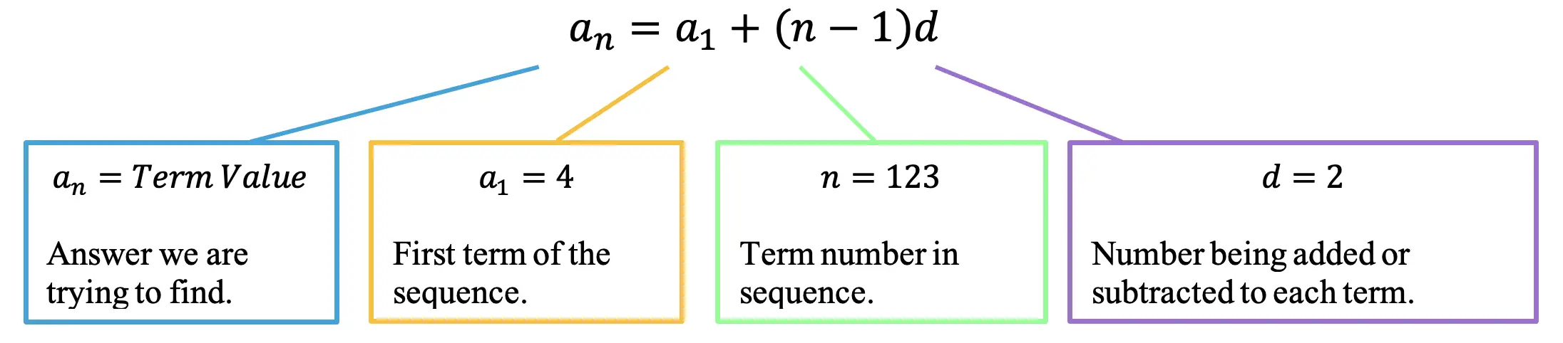
Step 2: Next, let’s write the arithmetic sequence formula and identify each part of our formula (First Term=4, Term number=123, common difference=2).
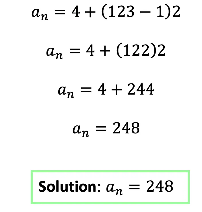
Step 3: Fill in our formula and solve with the given values.
Now let’s look at another example where we subtract the same number from each term in the sequence, making the common difference negative.
Step 1: First let’s identify the common difference between each previous term and each subsequent term of the sequence. Notice each term in the sequence is being subtracted by 3. Therefore, our common difference for this sequence is -3, negative, because we are subtracting.
Step 2: Next, let’s write the arithmetic sequence formula and identify each part of our formula (First Term=100, Term number=12, common difference=-3).
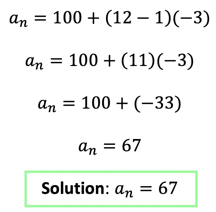
Step 3: Finally, let’s fill in our formula and solve with the given values.
Think you are ready to practice solving arithmetic sequences on your own? Try the following practice questions with solutions below:
Practice Questions:
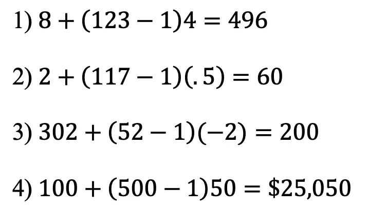
Find the 123rd term given the following sequence: 8, 12, 16, 20, 24, ….
Find the 117th term given the following sequence: 2, 2.5, 3, 3.5, …..
Find the 52nd term given arithmetic sequence: 302, 300, 298, …..
A software engineer charges $100 for the first hour of consulting and $50 for each additional hour. How much would 500 hours of the consultation cost?
Solutions:
Still got questions? No problem! Don’t hesitate to comment with any questions or check out the video above. Happy calculating! 🙂
Fun Fact!
Did you know that the arithmetic sequence formula can be considered an explicit formula? An explicit formula means that even though we do not know the other terms of a sequence, we can still find the unknown value of any term within the given sequence. For example, in the first example we did in this post (example #1), we wanted to find the value of the 123rd term of the sequence. We were able to do this by using the explicit arithmetic sequence formula, and most importantly, we were able to do this without finding the first 122 previous terms one by one…life is so much easier when there is an explicit arithmetic sequence formula in your life!
Other examples of explicit formulas can be found within the geometric sequence formula and the harmonic series.
Related Posts:
Looking to learn more about sequences? You’ve come to the right place! Check out these sequence resources and posts below. Personally, I recommend looking at the geometric sequence or finite arithmetic series posts next!
Still, got questions? No problem! Don’t hesitate to comment below or reach out via email. And if you would like to see more MathSux content, please help support us by following ad subscribing to one of our platforms. Thanks so much for stopping by and happy calculating!
Hey there math friends! In this post we will go over how and when to use synthetic division to factor polynomials! So far, in algebra we have gotten used to factoring polynomials with variables raised to the second power, but this post explores how to factor polynomials with variables raised to the third degree and beyond!
If you have any questions don’t hesitate to comment or check out the video below. Also, don’t forget to master your skills with the practice questions at the end of this post. Happy calculating! 🙂
What is Synthetic Division?
Synthetic Division is a shortcut that allows us to easily divide polynomials as opposed to using the long division method. We can only use synthetic division when we divide a polynomial by a binomial in the form of (x-c), where c is a constant number.
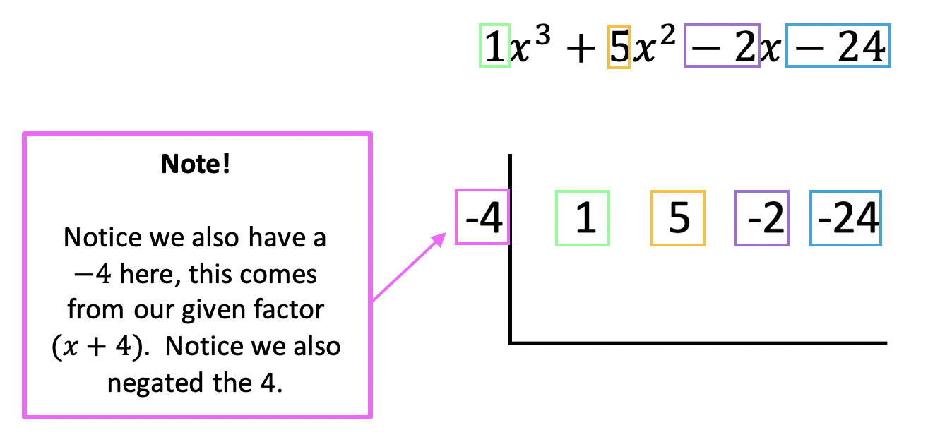
Example #1:
*Notice we can use synthetic division in this case because we are dividing by (x+4) which follows our parameters (x-c), where c is equal to 4.
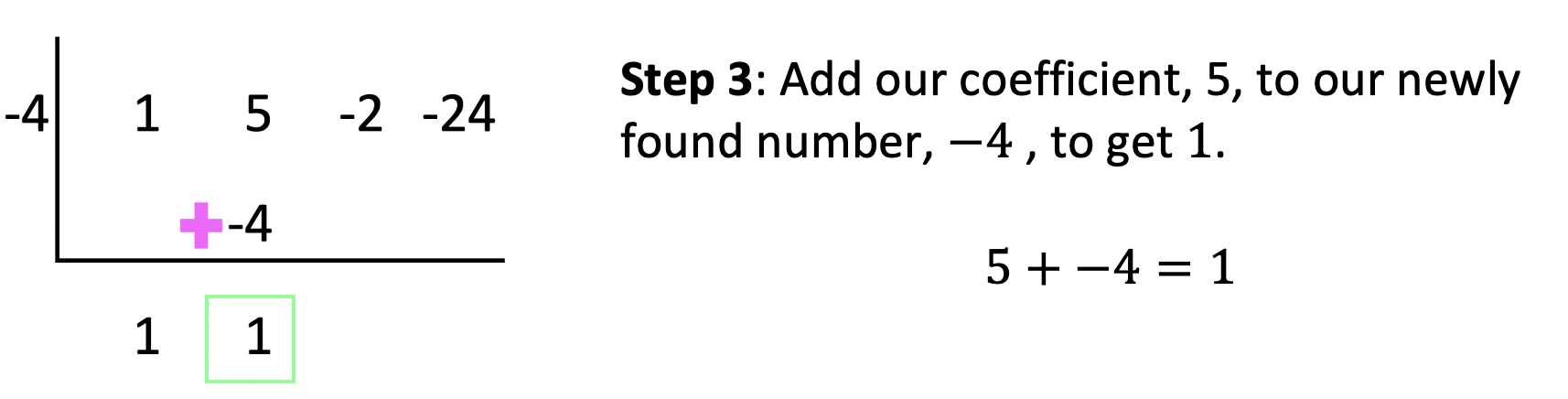
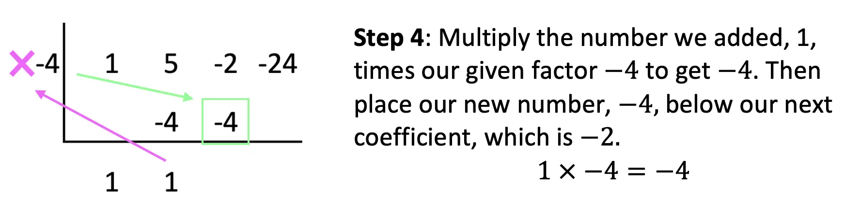
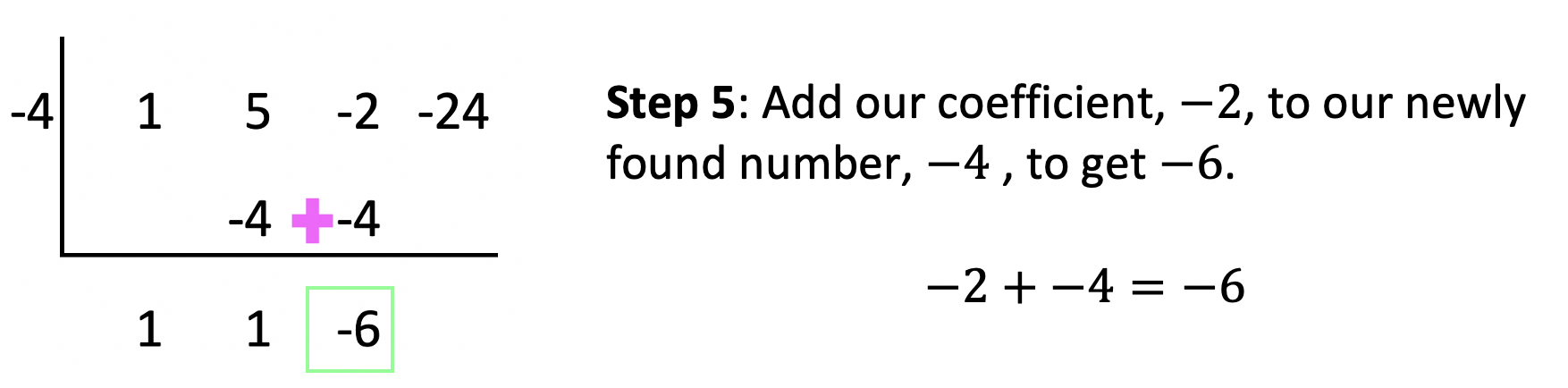
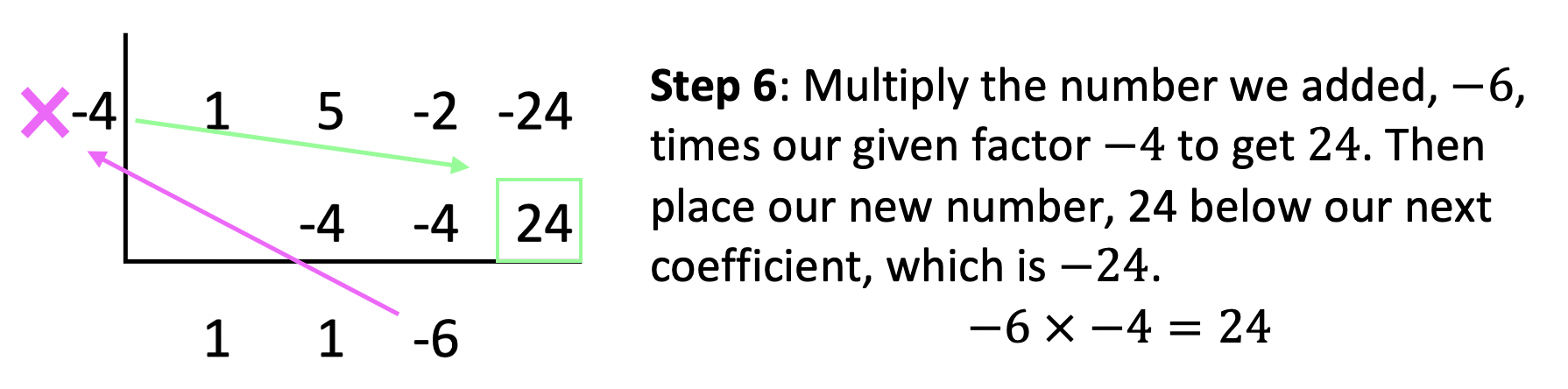
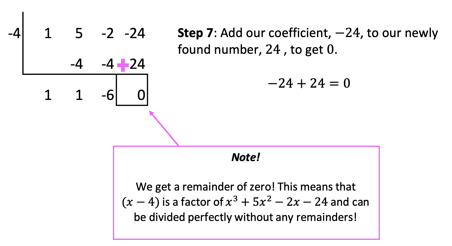
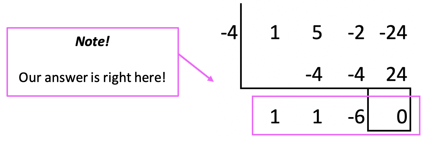
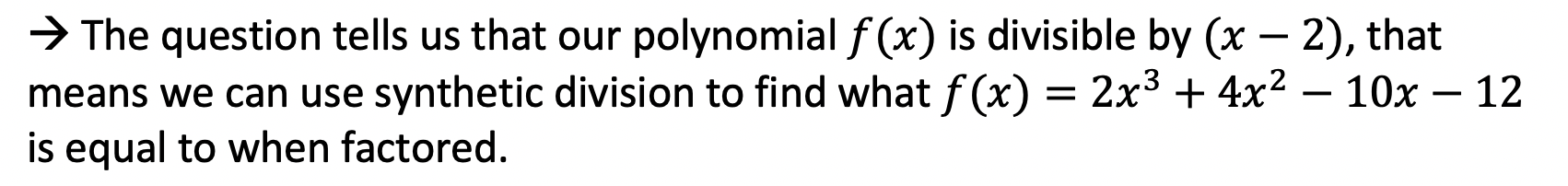
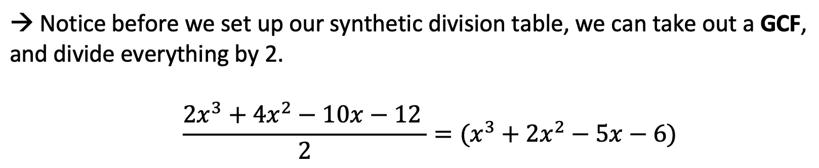
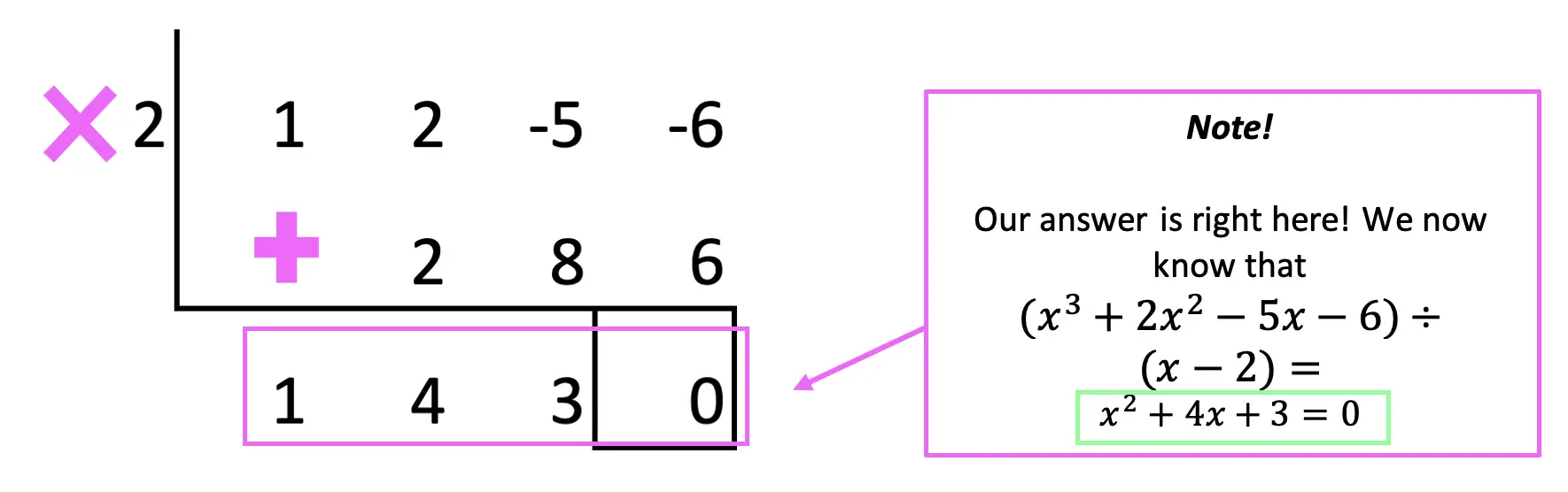
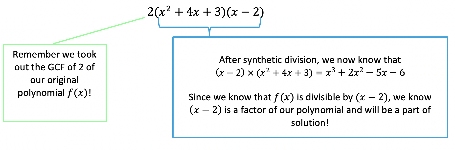
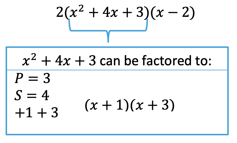
Example #2: Factoring Polynomials
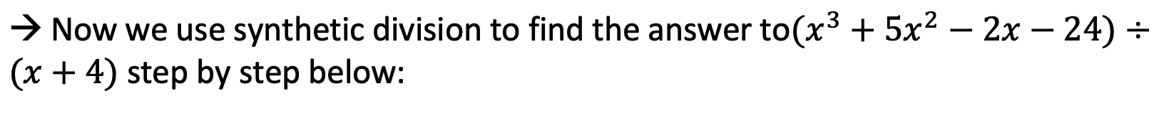
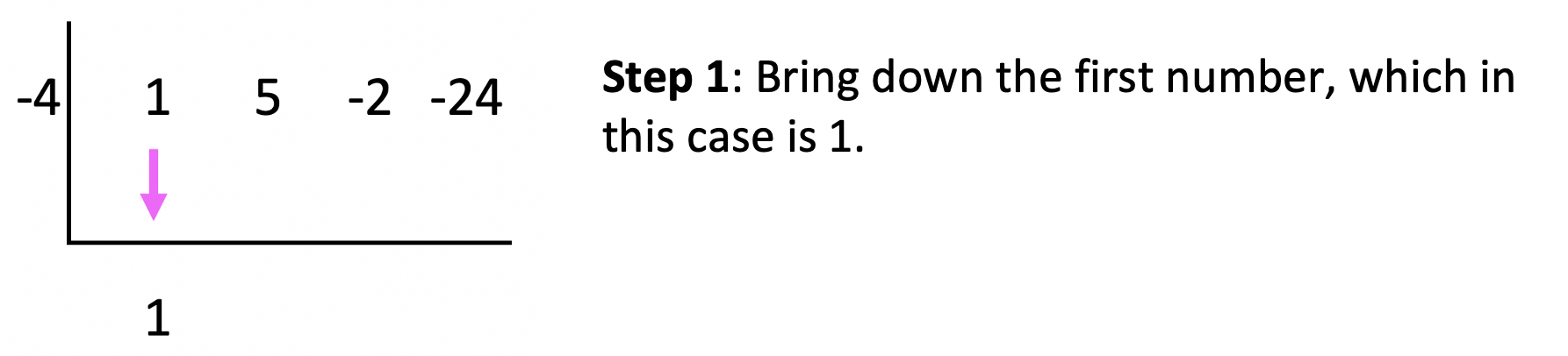
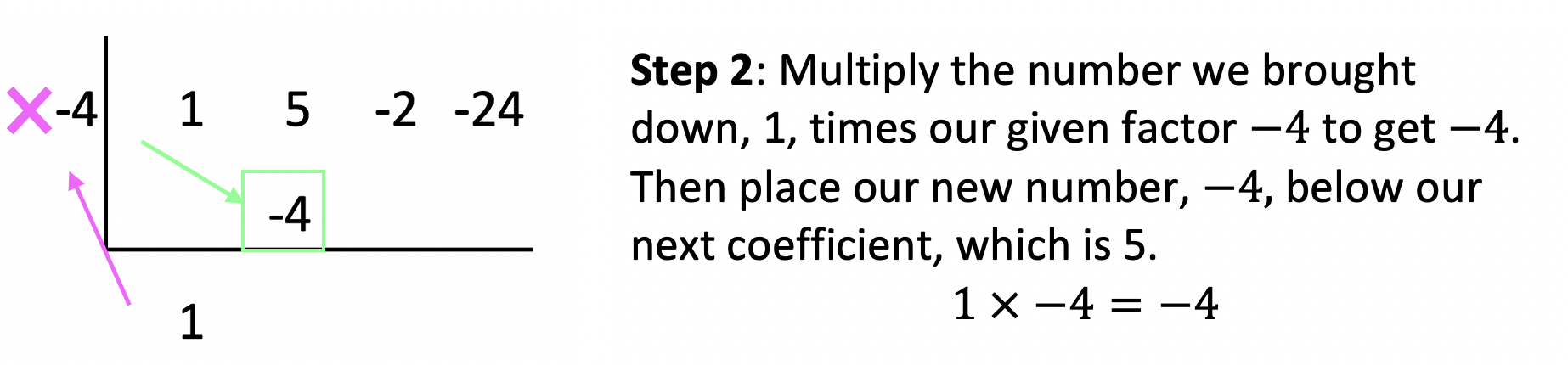
Let’s take a look at the following example and use synthetic division to factor the given polynomial:
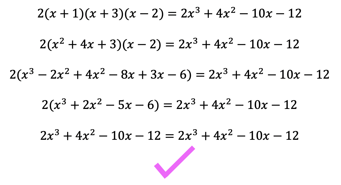
Check!
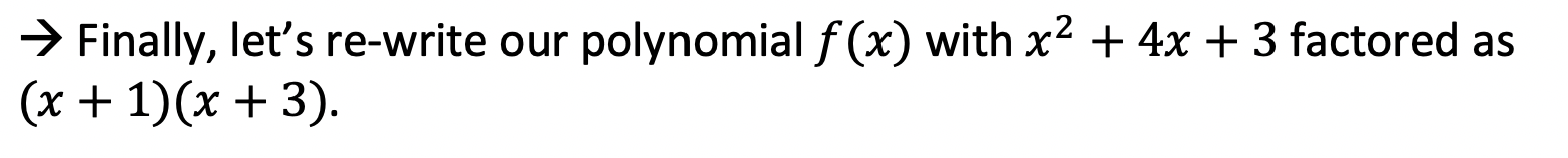
The great thing about these questions is that we can always check our work! If we wanted to check our answer, we could simply distribute 2(x+1)(x+3)(x-2) and get our original polynomial, f(x)=2x3+4x2-10x-12.
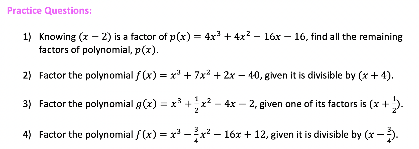
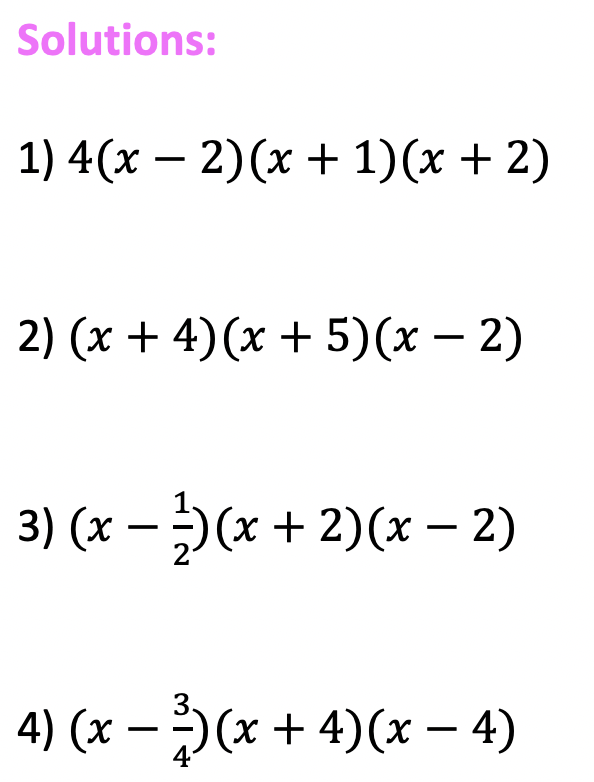
Try the practice problems on your own below!
Looking to brush up on how to divide polynomials the long way using long division? Check out this post here!
Still got questions? No problem! Don’t hesitate to comment with any questions or check out the video above. Happy calculating! 🙂